

Six machine learning methods (linear regression, logistic regression, extreme gradient boosting (XGBoost), support vector machine, K-nearest neighbours and artificial neural network) were used to predict/classify the hydraulic conductivity of conventional sodium bentonite (Na-B) geosynthetic clay liners (GCLs) to saline solutions or leachates. Data were collected from the literature and randomly divided into two groups – that is, 80% of the data were used to train machine learning models and the rest, 20%, were applied to evaluate model performance. Features that are known to affect the hydraulic conductivity of Na-B GCLs (e.g. mass per unit area of GCLs, monovalent and divalent cations, ionic strength (I), relative abundance of monovalent to divalent cations (RMD), swell index and effective stress) were employed to predict/classify the hydraulic conductivity of Na-B GCLs. Comparative analyses were conducted with seven subsets corresponding to the combination of different features, and the best model was determined through cross-validation. The results showed that XGBoost consistently had the best performance among all methods over all subsets of features for both regression and classification analyses. Subset 4, using the swell index, I, RMD, I2 × RMD, monovalent cations, divalent cations, effective stress and mass per unit area as features, outperformed all other six subsets in both regression analysis (R2 = 0.826) and classification analysis (accuracy = 0.887) in the out-of-sample tests.
Notation
- CD
concentration of divalent cations (mM)
- CM
concentration of monovalent cations (mM)
- I
ionic strength (mM)
- K
hydraulic conductivity of sodium bentonite (Na-B) geosynthetic clay liners (GCLs) (m/s)
- KDI
hydraulic conductivity of Na-B GCLs to deionised water (m/s)
mean value of (log(m/s))
measured hydraulic conductivity (log(m/s))
mean value of (log(m/s))
predicted hydraulic conductivity using machine learning models (log(m/s))
- N
total number of observations in the data set
- R2
coefficient of determination
- xmax
maximum value of the variable
- xmin
minimum value of the variable
- Zi
valence of the ith ion in solution
- σ
effective stress (kPa)
Introduction
Geosynthetic clay liners (GCLs) consist of a thin layer (5–10 mm) of sodium bentonite (Na-B) sandwiched between two layers of geotextiles. GCLs are widely used as hydraulic barriers in waste containment facilities due to their low permeability; thinness, which saves airspace; and ease of installation (Chen et al., 2018; Jo et al., 2001, 2005; Li et al., 2021a, 2023; Shackelford et al., 2000; Zainab et al., 2021). The primary mineral in Na-B GCLs is sodium (Na) montmorillonite, which has a large surface area, a high cation-exchange capacity and a high swelling potential (Bradshaw and Benson, 2014; Jo et al., 2001, 2005; Kolstad et al., 2004a; Lee et al., 2005; Li and Tian, 2022; Shackelford et al., 2000). Osmotic swelling of sodium montmorillonite reduces the pore size, resulting in a tortuous pathway for water flow and the low hydraulic conductivity of GCLs (e.g. <1 × 10⁻¹⁰ m/s) (Ashmawy et al., 2002; Athanassopoulos et al., 2015; Chen et al., 2018, 2019a; Gastelo et al., 2023; Guyonnet et al., 2005; Setz et al., 2017; Tian et al., 2016, 2019). However, the swelling of Na-B can be inhibited when exposed to leachates with high ionic strength (e.g. I > 300 mM), predominantly polyvalent cations and/or extreme pH conditions, leading to a large intergranular pore space and a high hydraulic conductivity of GCLs (>1 × 10⁻¹⁰ m/s) (Chen et al., 2019a; Di Emidio et al., 2015; Jo et al., 2001, 2005; Shackelford et al., 2000; Tian et al., 2016, 2019). It is important to determine whether a Na-B GCL can maintain low hydraulic conductivity to landfill leachates before applying it in the field.
Tremendous research has been conducted to investigate the hydraulic conductivity of Na-B GCLs to saline solutions or leachates from solid waste disposal facilities (Bradshaw et al., 2013, Chen et al., 2019a; Jo et al., 2001, 2005; Li et al., 2021b; Tian and Li, 2021; Tian et al., 2016; Zainab et al., 2021; Zhao et al., 2023). Tests are required to meet the termination criteria (e.g. hydraulic and chemical equilibria) according to ASTM D 6766 (ASTM, 2020) to reflect the long-term hydraulic conductivity of GCLs, which typically takes a very long time (e.g. months) (Jo et al., 2001, 2005; Scalia et al., 2014). Jo et al. (2005) reported that it took approximately 215 days for the hydraulic conductivity test of Na-B GCLs to 5 mM calcium chloride (CaCl2) solution to reach both hydraulic and chemical equilibria.
Alternatively, the swell index (SI) test (ASTM, 2019) is used as a quick index test to evaluate the chemical compatibility of Na-B GCLs with leachates. The hydraulic conductivity of Na-B GCLs is inversely related to the SI of bentonite – that is, Na-B GCL with a high SI in permeant solution can maintain a low hydraulic conductivity (Chen et al., 2018; Jo et al., 2001, 2005; Katsumi et al., 2008; Kolstad et al., 2004a; Lee et al., 2005). However, the relationship between the hydraulic conductivity of Na-B GCLs and the SI value is not unique. Na-B GCLs with the same SI may have different hydraulic conductivities. For example, Cruz (2021) reported that the hydraulic conductivity of Na-B GCLs to 10 mM calcium chloride was 5.8 × 10⁻¹¹ m/s with a SI of 24.0 ml/2 g. Chen et al. (2018) reported that Na-B GCLs showed a high hydraulic conductivity (e.g. 2.0 × 10⁻⁹ m/s) when permeated with synthetic coal combustion product (CCP) leachate (I = 48 mM), although the SI of Na-B was 24.0 ml/2 g.
Statistical models were also developed to predict the hydraulic performance of GCLs based on laboratory measurements. Kolstad et al. (2004a) proposed a linear regression equation for predicting the hydraulic conductivity of Na-B GCLs using ionic strength (I) and the relative abundance of monovalent to divalent cations (RMD) in the leachates as predictors. The proposed equation was valid for predicting the hydraulic conductivity of GCLs to leachates with I = 0.05–0.50 M and RMD < 2.0 mM1/2 at an effective stress of 20 kPa. Katsumi et al. (2007, 2008) proposed an equation for predicting the hydraulic conductivity of Na-B GCLs as a function of the SI. As discussed previously, the application of the SI as the sole factor may not accurately predict the hydraulic conductivity of Na-B GCLs. Empirical models were developed based on limited laboratory measurements, valid only to a limited extent (Katsumi et al., 2007, 2008; Kolstad et al., 2004a). Other factors such as effective stress and mass per unit area (MPUA) of Na-B GCLs also influence the hydraulic conductivity of Na-B GCLs. The empirical models may not provide accurate predictions of the hydraulic conductivity of Na-B GCLs permeated with saline solutions and leachates considering only the leachate properties or SI.
To date, machine learning (ML) approaches have been widely adopted in different domains in civil engineering (Chao et al., 2023a; Elbisy, 2015; Goli et al., 2022; Jiang et al., 2021; Kardani et al., 2022; Ozcoban et al., 2018; Rogiers et al., 2012; Salami et al., 2022; Samui, 2008; Shahin et al., 2002; Zhang et al., 2021). Many ML algorithms, such as artificial neural networks (ANNs), support vector machines (SVMs) and K-nearest neighbours (KNN), have been used to estimate the hydraulic conductivity of soil. Rogiers et al. (2012) applied multiple linear regression (MLR) and ANN models to estimate the saturated hydraulic conductivity of soil using grain-size distribution data. The ANN model proved to be more accurate than the MLR model, with greater accuracy in predicted hydraulic conductivity (e.g. R2: 0.93 against 0.89). Das et al. (2012) applied ANN and SVM models to predict the field hydraulic conductivity of clay liners based on in situ test results. The input of the models included the liquid limit, plastic limit, percentage fines content, moisture content, dry density, weight of the compactor, lift thickness and number of lifts. Raja and Shukla (2021) combine the grey-wolf optimisation (GWO) and ANN algorithms (ANN–GWO) to predict the settlement of a geosynthetic-reinforced soil foundation (GRSF). The results showed that the proposed model (ANN–GWO) predicts the settlement of a GRSF with higher accuracy compared with an ANN model (root mean square error: 0.612 against 0.774; R2: 0.962 against 0.943).
The objective of this paper is to explore and develop an ML-based framework to predict the hydraulic conductivity of Na-B GCLs to leachates. Six ML algorithms – namely, linear regression, logistic regression, extreme gradient boosting (XGBoost), SVM, KNN and ANN – are applied and compared in this study. Two types of target (output) variables are investigated according to two tasks: (a) prediction of the hydraulic conductivity of GCLs and (b) classification of the status of hydraulic conductivity based on the threshold value (i.e. ‘success’ if ≤1 × 10⁻¹⁰ m/s; ‘failure’, otherwise). The input features of the models include leachate properties (I, RMD, concentrations of monovalent and divalent cations), MPUA of GCLs, SI and effective stress. The model developed in this study can be used to select appropriate Na-B GCLs to manage leachates from solid waste disposal facilities.
Background
Method for predicting the hydraulic conductivity of Na-B GCLs
Swell index
Numerous studies have shown that there exist relationships between the SI and hydraulic conductivity of Na-B GCLs (Chen et al., 2018; Guyonnet et al., 2005; Jo et al., 2001, 2005; Katsumi et al., 2008; Kolstad et al., 2004a; Lee et al., 2005; Wireko et al., 2020). For Na-B GCLs, a hydraulic conductivity <1.0 × 10⁻¹⁰ m/s generally correlates with SI >20 ml/2 g at low effective stress and without prehydration (Scalia et al., 2018).
However, the relationship between the hydraulic conductivity of Na-B GCLs and the SI is not trivial at low effective stress, as shown in Figure 1 (which compiles all available data in the literature). The hydraulic conductivity of Na-B GCLs to saline solutions or leachates is higher than 1 × 10⁻¹⁰ m/s when the swelling of bentonite is < 12 ml/2 g, whereas Na-B GCLs can maintain a low hydraulic conductivity (e.g. <1 × 10⁻¹⁰ m/s) when the SI is higher than 30 ml/2 g. When the SI of Na-B falls into the range between 12 and 30 ml/2 g, no conclusion can be made on whether Na-B GCLs can maintain a hydraulic conductivity lower than the threshold or not.
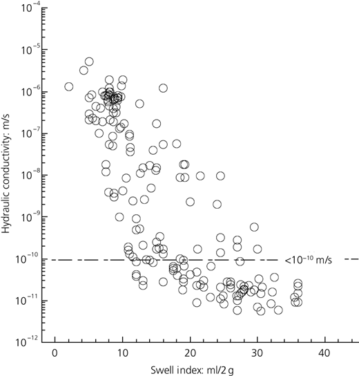
Hydraulic conductivity of Na-B GCLs to saline solutions or leachates as a function of the SI in the literature (note: data from Ashmawy et al. (2002), Jo et al. (2001, 2005), Shan and Lai (2002), Kolstad et al. (2004a, 2004b), Lee et al. (2005), Li et al. (2021a, 2021b), Lin et al. (2000), Katsumi et al. (2007, 2008), Meer and Benson (2007), Benson and Meer (2009), Bradshaw and Benson (2014), Bradshaw et al. (2016), Electric Power Research Institute (EPRI, 2014), Scalia et al. (2014), Salihoglu (2015), Tian et al. (2016, 2019), Setz et al. (2017), Chen et al. (2018, 2019a), Wang et al. (2019), Cruz (2021), Wireko and Abichou (2021), Wireko et al. (2022), Zainab et al. (2021))
Hydraulic conductivity of Na-B GCLs to saline solutions or leachates as a function of the SI in the literature (note: data from Ashmawy et al. (2002), Jo et al. (2001, 2005), Shan and Lai (2002), Kolstad et al. (2004a, 2004b), Lee et al. (2005), Li et al. (2021a, 2021b), Lin et al. (2000), Katsumi et al. (2007, 2008), Meer and Benson (2007), Benson and Meer (2009), Bradshaw and Benson (2014), Bradshaw et al. (2016), Electric Power Research Institute (EPRI, 2014), Scalia et al. (2014), Salihoglu (2015), Tian et al. (2016, 2019), Setz et al. (2017), Chen et al. (2018, 2019a), Wang et al. (2019), Cruz (2021), Wireko and Abichou (2021), Wireko et al. (2022), Zainab et al. (2021))
Empirical model
Kolstad et al. (2004a) developed an empirical equation for predicting the hydraulic conductivity of Na-B GCLs (MPUA = 4.3 kg/m2) based on the ionic strength (I) and RMD of the inorganic solution. The equation was developed based on 31 hydraulic conductivity test observations (data set A from Table 1) using stepwise regression, as shown in the following equation:
Empirical models for predicting the hydraulic conductivity of Na-B GCLs
| Empirical model | Data set | Number of data | Permeant solutions | Effective stress: kPa | MPUA: kg/m2 | a | b | c | d | R2 |
|---|---|---|---|---|---|---|---|---|---|---|
(Kolstad et al., 2004a) | Aa | 31 | Saline solutions | 20 | 4.3 | 0.965 | −0.976 | 0.0797 | 0.251 | 0.967 |
| Bb | 82 | Saline solutions, synthetic CCP leachates, MSW leachates | 20 | 3.6–5.1 | 0.880 | −0.740 | 0.103 | 0.221 | 0.514 | |
(Katsumi et al., 2007) | Cc | 40 | DI water, saline solutions, MSW leachate | 20–30 | 4.73 | −0.310 | 8.690 | 3.09 × 10⁻¹¹ | N/A | 0.830 |
| Dd | 248 | DI water, saline solution, MSW, CCP, LLW leachates, bauxite liquor | 20–30 | 3.6–6.4 | −0.070 | 28.220 | 5.20 × 10⁻¹² | N/A | 0.595 |
Data from Kolstad et al. (2004a)
Data from Jo et al. (2001), Kolstad et al. (2004a), Lee et al. (2005), EPRI (2014), Scalia et al. (2014), Bradshaw et al. (2016), Chen et al. (2018, 2019a), Tian et al. (2019), Cruz (2021), Wireko and Abichou (2021) and Zainab et al. (2021)
Data from Katsumi et al. (2007).
Data from Lin et al. (2000), Jo et al. (2001), Ashmawy et al. (2002), Kolstad et al. (2004a), Lee et al. (2005), Katsumi et al. (2007, 2008), Meer and Benson (2007), Benson and Meer (2009), Scalia et al. (2014), Bradshaw et al. (2014), EPRI (2014), Salihoglu (2015), Tian et al. (2016, 2019), Setz et al. (2017), Chen et al. (2018, 2019a), Cruz (2021), Li et al. (2021a, 2021b), Wireko and Abichou (2021), and Zainab et al. (2021) CCP, coal combustion product; DI, deionised; LLW, low-level radioactive waste; MSW, municipal solid waste
Equation 1 is linear in I and RMD, and the product I2 × RMD reflects that the sensitivity to RMD varies non-linearly with ionic strength. The equation is valid for I = 0.05–0.50 M and RMD < 2.0 M1/2 and at 20 kPa (Kolstad et al., 2004a).
A new data set B (containing 82 hydraulic conductivity tests) was created by combining the data reported by Kolstad et al. (2004a) (31 tests) and additional data set (51 tests) from the literature (Table 1). The fitting parameters of Equation 1 for data set B were obtained by regression analysis, as shown in Table 1. R2 decreased to 0.514. Most of the predicted hydraulic conductivity of Na-B GCLs for data set B fell within two orders of magnitude in comparison with the measured value (Figure 2(a)). The low prediction accuracy reflected the limitation of Equation 1, indicating that factors other than ionic strength and RMD might affect the hydraulic conductivity of GCLs.
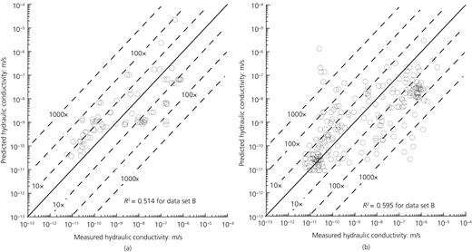
Predicted hydraulic conductivity plotted against measured hydraulic conductivity (a) as a function of ionic strength and RMD using the method proposed by Kolstad et al. (2004a) and (b) as a function of the SI using the method proposed by Katsumi et al. (2007)
Predicted hydraulic conductivity plotted against measured hydraulic conductivity (a) as a function of ionic strength and RMD using the method proposed by Kolstad et al. (2004a) and (b) as a function of the SI using the method proposed by Katsumi et al. (2007)
Katsumi et al. (2007, 2008) proposed another empirical equation for predicting the hydraulic conductivity Na-B GCLs as a function of the SI. The equation was developed based on 40 hydraulic conductivity tests at 29.4 kPa effective stress (Table 1, data set C) (Katsumi et al., 2007, 2008), as shown in the following equation:
Equation 2 can be used under an effective stress of 20–30 kPa. A new data set D (248 tests) was compiled including the hydraulic conductivity of Na-B GCLs to saline solutions and leachates at 20–30 kPa effective confining stress (Table 1). The R2 of Equation 2 using data set D decreased to 0.595. The predicted hydraulic conductivity of Na-B GCLs primarily fell within 1000 times (three orders of magnitude) to the measured value, as shown in Figure 2(b). The low R2 of Equation 2 illustrates that the prediction of hydraulic conductivity of the Na-B GCLs as a function of the SI is insufficient and inaccurate, as discussed in the previous section.
The two empirical models showed poor performance in predicting the hydraulic conductivity of Na-B GCLs permeated with saline solutions and leachates and thus may not provide accurate predictions for selecting appropriate Na-B GCLs to manage landfill leachates. It is important to develop a more accurate model for predicting the hydraulic conductivity of Na-B GCLs. Therefore, this study developed an ML-based framework for predicting the hydraulic conductivity of Na-B GCLs to leachates using MPUA, leachate properties (e.g. I and RMD), effective stress (σ) and SI.
ML algorithms
ML has been widely applied in geotechnical engineering due to its capability and flexibility to characterise complex relationships between variables. Supervised ML approaches can be broadly categorised into two classes – regression and classification, where the regression model aims to predict the numerical value of the target variable and the classification model aims to predict the categorical level of the target variable. In this study, six popular ML approaches were adopted and compared – namely, linear regression, logistic regression, XGBoost, SVM, KNN and ANN. Linear regression can be used only for regression tasks, logistic regression is used only for classification tasks, while the remaining four can be used for both regression and classification tasks. To be self-contained, a brief introduction to XGBoost, SVM, KNN and ANN are described in the following sections, while the descriptions of linear and logistic regression models are skipped since they are well known.
Extreme gradient boosting
XGBoost is an ensemble learning algorithm based on classification and regression trees (Carts). A single Cart is considered a weak ML model – that is, it is not a competitive model with a high prediction accuracy (James et al., 2013). To improve the model performance, many ensemble ML models are developed based on Carts using the bagging or boosting approach. For instance, a random forest is developed based on the bagging approach and consists of multiple Carts. Further developed from random forests, XGBoost is an ensemble learning algorithm that uses a gradient boosting framework with higher computational efficiency than a random forest model with a weighted quantile design (Chen and Guestrin, 2016). The idea of XGBoost is to add trees continuously and perform feature splitting to grow a tree. The new tree learns a new Cart function to fit the residual of the last prediction. When the training process is completed, a specified number of trees are obtained as outcomes. Each of the learned trees corresponds with a leaf node and a prediction score. The final predicted value is calculated as the weighted sum of the scores across all trees. The XGBoost method shows advantages over logistic regression in terms of accuracy and predictive power. As an ensemble method that combines multiple decision trees, XGBoost captures non-linear patterns in the data that a logistic regression model may overlook. Furthermore, through gradient boosting, XGBoost reduces its error rate with each iteration, leading to more precise predictions. Additionally, XGBoost efficiently handles large, high-dimensional data sets without feature selection, making it suitable for demanding ML tasks. Although its black-box nature may be perceived as a drawback, the exceptional accuracy and predictive power of XGBoost outweigh this lack of interpretability. Relative influence was employed to obtain the importance for each predictor. At each split in each tree, the improvement in the split criterion (mean squared error (MSE) for regression, accuracy for classification) was computed. Then, the average of the improvement made by each variable across all the trees can be calculated. The variables with the largest average decrease in MSE or increase in accuracy were considered most important.
Support vector machine
An SVM is an ML model that can be utilised for classification and regression analysis (Cortes and Vapnik, 1995). The basic idea of SVMs comes from the maximum margin classifier, which is a classification method based on selecting the hyperplane that can maximise the interval between each class. More specifically, for two-class classification analysis, the SVM algorithm maps training observations to points in space and then maximises the hyperplanes between the two categories through a fixed kernel function. The new input observations are mapped into the same space, and which side of the gap the new mapped points belong to is analysed. SVMs can also be applied in regression analysis resulting from the support vector regression (SVR) model. Unlike linear regression models that minimise the error between the actual and predicted values, SVR can fit the optimal line within a threshold of values called the epsilon-insensitive tube. SVMs can capture non-linear relationships among the variables by adopting different kernel functions, such as linear, polynomial and radial basis kernels (Chao et al., 2023b).
K-nearest neighbours
KNN is a non-parametric ML approach that can be used for regression and classification analysis, where K is a positive integer specified by the user (Anava and Levy, 2016). The idea behind KNN is to predict/classify the observation according to its most similar neighbours. For both cases, the input training data are assumed to contain K-closest neighbours. For the case of classification, the output object is classified by the plurality vote of the neighbours. The output case is predicted by the average value of its KNN in the training data set for the regression case. The number of K is the only hyperparameter that needs to tune in the model-training process.
Artificial neural networks
ANNs are a supervised learning algorithm that is the basis of deep learning research (Chen et al., 2019b). The name of ANNs are inspired by the human brain, mimicking the way that biological neurons signal to one another. ANNs comprise node layers, including an input layer, at least one hidden layer and an output layer. Each node in the network has a threshold value and weight. If the output of a node is over the given threshold value, the node become active and passes the data to the next layer. If the node cannot be activated by the output, the node will not send data to the next layer. The output of a node is obtained by the activation function based on the inputs of the node. For regression analysis, the output layer provides continuous results based on one node. For classification analysis, the output is classified in one of the classes.
Framework of hydraulic conductivity prediction
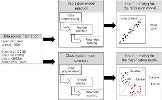
The proposed framework for predicting hydraulic conductivity is shown in Figure 3. Two different approaches were considered in the proposed procedure: one was regression and the other one was classification. The two approaches were conducted independently. The procedure consists of three modules – namely, data source integration, model selection and out-of-sample performance evaluation. The tasks to be completed in each module are summarised as follows.
- ▪
Data source integration. Multiple data sets were collected from the existing literature and were integrated according to the feature variables.
- ▪
Model selection. Different ML models were constructed using training data, and the best model (with features) was selected through a k-fold cross-validation (CV) procedure.
- ▪
Performance evaluation. The value (or success/failure status) of the hydraulic conductivity of Na-B GCLs to saline solution or leachate was predicted using the holdout testing data to evaluate the proposed model performance with the selected model.
Data preparation
The data used in this study are collected from 22 papers from the years 2000 to 2022, including those on CCP, municipal solid waste (MSW), low-level radioactive waste and MSW incineration ash landfill leachates, which represent the typical leachates in landfills (Benson and Meer, 2009; Bradshaw and Benson, 2014; Bradshaw et al., 2016; Chen et al., 2018; Cruz, 2021; EPRI, 2014; Jo et al., 2001; Katsumi et al., 2007; Kolstad et al., 2004a; Lee et al., 2005; Li et al., 2021a, 2021b; Meer and Benson, 2007; Salihoglu, 2015; Scalia et al., 2014; Setz et al., 2017; Tian et al., 2016, 2019; Wang et al., 2019; Wireko and Abichou, 2021; Wireko et al., 2022; Zainab et al., 2021). Table 2 summarises the minimal, median, mean and maximal values of each variable. The hydraulic conductivity of Na-B GCLs in the data set ranged from 1.8 × 10⁻¹² to 5.2 × 10⁻⁶ m/s. The SI in the data set ranged from 2.0 to 35.6 ml/2 g, and the MPUA of Na-B GCLs ranged from 3.6 to 6.4 kg/m2. The effective stress in the data set ranged from 20 to 500 kPa, and most of the effective stresses were lower than 40 kPa (63.9%).
Summary of data variables
| Variable | Unit | Min. | Median | Mean | Max. |
|---|---|---|---|---|---|
| Hydraulic conductivity, K | m/s | 1.8 × 10⁻¹² | 1.1 × 10⁻⁹ | 1.8 × 10⁻⁷ | 5.2 × 10⁻⁶ |
| Monovalent cations | mM | 0.0 | 62.6 | 249.5 | 4638.7 |
| Divalent cations | mM | 0.0 | 18.5 | 89.2 | 1000.0 |
| Ionic strength, I | mM | 0.02 | 171.7 | 496.2 | 4676.0 |
| RMD | M0.5 | 0.00 | 0.65 | 14.59 | 100.00a |
| Effective stress, σ | kPa | 20.0 | 20.0 | 97.6 | 500.0 |
| MPUA | kg/m2 | 3.6 | 4.0 | 4.2 | 6.4 |
| SI | ml/2 g | 2.0 | 13.5 | 14.3 | 35.6 |
100 indicates infinity observations of RMD (∞)
I, ionic strength; MPUA, mass per unit area; RMD, relative abundance of monovalent to divalent cations; SI, swell index; σ, effective stress
The entire data set consisting of 308 observations from field experiments of infiltration process were separated randomly into two groups, which were denoted as training and testing data sets. For the train–test split ratio, there was no clear guidance on what ratio was best or optimal for a given data set (Joseph, 2022). A widely used train–test split ratio was 80:20, which meant 80% of the data were for training and 20% are for testing. Other train–test split ratios such as 70:30, 60:40 and 50:50 were also used in practice. The 80:20 split draws its justification from the well-known Pareto principle (Sanders, 1987). The selection of the size of the training data set primarily depended on the complexity of the model. Previous research has shown that the number of the data sets should be at least ten times that of the features for small models (Harrell et al., 1996; Peduzzi et al., 1996). In the present study, the training data set was composed of 246 observations, and the number of features ranged from 2 to 8. The size of the training data set in this study met this rule of thumb. In this sense, the 80:20 ratio was adopted in this study. The training data set contained 246 observations (∼80% of the total data), while the testing data had 62 observations (the remaining ∼20% of the total data) (Sanders, 1987). To validate the model generalisation ability, the 70:30 ratio was also compared in this study. The input parameters (features) included monovalent cations, divalent cations, I, RMD, I2 × RMD, effective stress, MPUA and SI. Both regression and classification models were investigated. For the regression model, the numerical value of hydraulic conductivity of GCL was used as the target variable. For the classification model, the status of hydraulic conductivity – that is, success (when the hydraulic conductivity was ≤1 × 10⁻¹⁰ m/s) or failure (when the hydraulic conductivity was >1 × 10⁻¹⁰ m/s) – was employed as the target variable.
Data preprocessing
Data preprocessing was conducted before the training procedure to improve the performance of ML models. When the concentration of monovalent cations in calcium chloride solution and that of divalent cations in sodium chloride (NaCl) solution equal zero, the zero values of monovalent cations and divalent cations in the leachate composition were replaced by 0.001. Logarithm transformation of hydraulic conductivity, monovalent cations, divalent cations and ionic strength was performed taken to convert the data to be more normally distributed. Then, to rescale all independent variables into the same range, min–max normalisation was performed using the following equation:
where xmin and xmax were the minimum and maximum values of the variable, respectively. Finally, data sets were randomly divided into two subsets: 80% as the training set and 20% as the holdout testing set. The training set was used to build and tune ML models, and the testing set was used to evaluate the performance of the built models.
Model training
The optimal model for each ML algorithm was studied through k-fold CV during the training process. At the beginning of the k-fold CV approach, the training data were randomly and evenly divided into k folds. Then, the first fold was considered the validation set and the remaining k − 1 folds were used to build a learning model. The validation fold was employed to evaluate the performance of the obtained model. The process was repeated k times. Each time, a different fold of data was considered a validation set and a model was trained with the remaining folds. For each round, the MSE (or accuracy) was calculated in the validation data. Then, the k-fold CV estimate was obtained by taking the average over the k MSEs (or accuracy). The value of k was set as 5 in this study (i.e. fivefold CV).
Two assignments were considered in the model-training process: feature selection and parameter tuning. Feature selection could improve the model prediction accuracy and model interpretability. In this study, the subset selection approach was used to conduct feature selection progress. Based on the previous literature, key variables that are known to affect the hydraulic conductivity of Na-B GCLs to saline solution and leachate were divided and combined to create feature subsets, as listed in Table 3. The variables can be classified into four categories: (a) GCL properties (MPUA); (b) leachate properties (e.g. monovalent and divalent cations, I, RMD); (c) effective confining stress; and (d) SI. Overall, seven subsets corresponding to different combinations of features were evaluated in this study, which can be divided into three comparative categories. Subsets 1 and 2 consider MPUA effective confining stress with various combinations of leachate properties (Table 3). The comparison between subsets 1 and 2 can illustrate the significance of parameters within leachate properties. In comparison with subsets 1 and 2, one additional parameter (e.g. SI) was evaluated in subsets 3–5. The comparison between these two sets can reveal the importance of SI on predicting the hydraulic conductivity of Na-B GCLs. Subsets 6 and 7 were compared to evaluate the accuracy of the prediction of the hydraulic conductivity of Na-B GCLs based on the three parameters of SI, MPUA and effective confining stress.
Subsets of the predictors
| Subset 1 | MPUA, σ, monovalent cations, divalent cations, I, RMD, I2 × RMD |
| Subset 2 | MPUA, σ, I, RMD |
| Subset 3 | MPUA, σ, monovalent cations, divalent cations, I, RMD, SI |
| Subset 4 | MPUA, σ, monovalent cations, divalent cations, I, RMD, I2 × RMD, SI |
| Subset 5 | MPUA, σ, I, RMD, SI |
| Subset 6 | MPUA, σ, SI |
| Subset 7 | σ, SI |
I, ionic strength; MPUA, mass per unit area; RMD, relative abundance of monovalent to divalent cations; SI, swell index; σ, effective stress
Moreover, when training the model, some hyperparameters of the ML models cannot be directly estimated through an algorithm. A commonly used method to obtain the optimal hyperparameters is grid search, which can exhaustively search a designated subset of the hyperparameter space of the ML model. In the training process, a grid search algorithm was used to find the optimal hyperparameters for each ML model through fivefold CV over each proposed feature subset (James et al., 2013). The detailed ML model parameter settings and employed packages are listed in the Appendix (which also includes Tables 8–12).
Evaluation metric and testing
Evaluation metric for the regression model
The performance of regression models was evaluated using five metrics: MSE, coefficient of determination (R2), mean absolute error (MAE), mean absolute percentage error (MAAPE) and refined Willmott index (RWI). Denoting and , MSE and R2 are obtained as follows:
where N is the number of observations; is the predicted result using ML models; represents the mean value of ; is the measured hydraulic conductivity; and represents the mean value of . The best model performance is marked by high R2 and RWI and low MSE, MAE and MAAPE values.
Evaluation metric for the classification model
Two metrics – accuracy and area under the curve (AUC) – were used to evaluate the performance of the classification models. Accuracy denotes the overall proportion of observations that are correctly classified. The accuracy metric is primarily used to evaluate performance and select the best model. The mathematical expression for accuracy is as follows:
where N represents the total number of observations in the data set. The true positive (TP) expresses the number of positive class observations correctly classified into the positive class by the ML model (Kmeasured, Kpredicted ≤ 1 × 10⁻¹⁰ m/s). The true negative (TN) indicates negative class observations correctly classified into the negative class (Kmeasured, Kpredicted > 10−10 m/s).
The AUC value is also reported to measure the overall performance of the classification model, which represents the area under the receiver operating characteristic curve. The AUC is an evaluation metric that works only for two-class classification analysis. For binary samples (positive and negative), the AUC value represents the probability that the chance that a positive observation is classified into a positive class is larger than the chance that this observation is classified as a negative class. The range of the AUC is between 0.5 and 1. When the AUC value is equal to 1, the model can perfectly classify the given samples. When the AUC value is equal to 0.5, the model has no power to conduct prediction; and therefore, has no application value.
Regression analysis results
Model comparison
The model performance of all training models (e.g. MSE, R2, MAE, MAAPE, RWI) across subsets 1–7 is shown in Figure 4. The models with advanced algorithms such as XGBoost, SVM, KNN and ANN outperformed the linear regression model. For each subset, the XGBoost model had consistently the best performance by giving the smallest MSE, MAE and MAAPE and highest RWI and R2 in comparison with those of the other four models. For instance, the MSE of XGBoost for subset 3 was 0.126, which was 1127.8, 761.9, 438.9% and 513.5% lower than those of linear regression, SVM, KNN and ANN, respectively. The R2 of subset 3 by the XGBoost method was 0.962, which was 17.5–40.8% higher than those of the other four methods. The RWI of subset 3 was also 18.5–63.9% higher than those of the other four methods. Therefore, these results showed that XGBoost was the most accurate method in predicting the hydraulic conductivity of Na-B GCLs to saline solutions or leachates. Hereafter, the discussion focuses on the comparison among subsets 1–7 using XGBoost methods. The results for the 70:30 ratio show similar (although slightly poorer) performance in the training data set as those for the 80:20 ratio. The subsequent discussion is based on the 80:20 ratio.
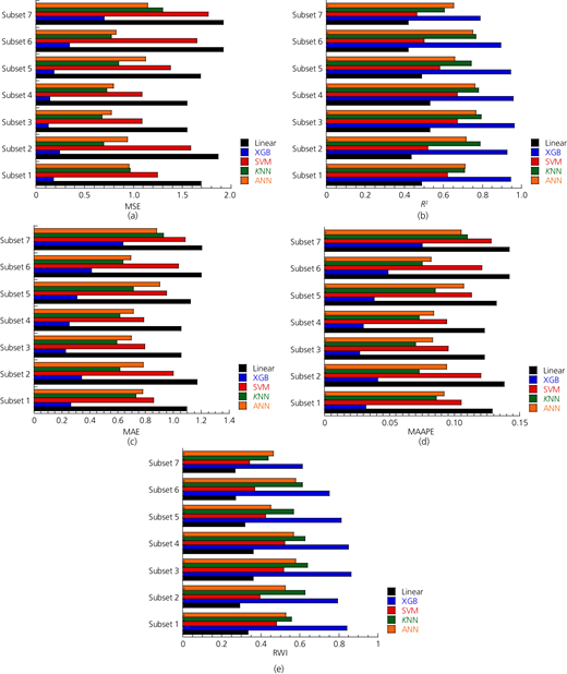
Model performance on the training data set by regression analysis using linear regression, XGB, SVM, KNN and ANN: (a) MSE; (b) R2; (c) MAE; (d) MAAPE; (e) RWI
Model performance on the training data set by regression analysis using linear regression, XGB, SVM, KNN and ANN: (a) MSE; (b) R2; (c) MAE; (d) MAAPE; (e) RWI
The model performance of the training data set with subsets 1–7 by the XGBoost method is shown in Table 4. Subsets 1 and 2, considering MPUA, leachate properties and effective stress factor, illustrated great performance in terms of low MSE, MAE and MAAPE and high R2 and RWI. Subsets 3–5 contained the same features as subsets 1 and 2 correspondingly but with one additional feature - the SI. With the SI, the performance of subsets 3–5 improved on that of subsets 1 and 2 with MSE ranging from 0.126 to 0.186 and R2 from 0.944 to 0.962. Subsets 6 and 7, ignoring leachate properties, had the worst performance in predicting the hydraulic conductivity of Na-B GCLs – that is, in terms of high MSE, MAE and MAAPE and low R2 and RWI – in comparison with those of subsets 1–5.
Model performance for training data using regression analysis (XGBoost algorithm)
| Subset | MSE: log2(m/s) | R2 | MAE: log(m/s) | MAAPE | RWI |
|---|---|---|---|---|---|
| 1 | 0.183 | 0.944 | 0.264 | 0.032 | 0.840 |
| 2 | 0.244 | 0.926 | 0.340 | 0.041 | 0.793 |
| 3 | 0.126 | 0.962 | 0.227 | 0.027 | 0.862 |
| 4 | 0.141 | 0.957 | 0.251 | 0.030 | 0.848 |
| 5 | 0.186 | 0.944 | 0.310 | 0.038 | 0.812 |
| 6 | 0.346 | 0.895 | 0.411 | 0.049 | 0.751 |
| 7 | 0.699 | 0.788 | 0.637 | 0.075 | 0.614 |
Empirical equations were developed using the linear regression method based on subsets, as shown in Table 10. The model with subset 4 (Equation 10) by the linear regression method outperformed the other six Subsets (Table 11), considering the leachate properties, GCL properties, SI and effective stress.
where K is the hydraulic conductivity (m/s); σ is the effective stress (kPa); MPUA is the mass per unit area (kg/m2); CM is the concentration of monovalent cations (mM); and CD is the concentration of divalent cations (mM).
The R2 of Equation 10 was 0.531, which was much lower than that developed by the XGBoost method (e.g. 0.531 against 0.957). Equation 10 was supposed to be linear in all eight parameters (e.g. σ, MPUA, SI, CM, CD, I, RMD, I2RMD) in the linear regression method. The logarithm of hydraulic conductivity was reported to be not linear with parameters such as SI and effective stress (e.g. log K ∼ exp(SI), log K ∼ σ0.5), which resulted in poorer model performance (Bradshaw et al., 2013; Katsumi et al., 2007, 2008). Equation 10 could be calculated also to classify the status of the hydraulic conductivity of Na-B GCLs (e.g. ≤10−10 or >10−10 m/s) but with a lower accuracy (0.842). It is important to develop a tool (e.g. classification model) to expedite the screening process for identifying qualified Na-B GCLs to manage specific leachates (e.g. ≤1 × 10⁻¹⁰ m/s).
Feature importance analysis
XGBoost is an ensemble ML method that can evaluate the comparative contribution (or relative importance) of each feature in predicting the target variable. A feature with higher relative importance indicates a greater contribution to predicting the target value. This section analyses the feature importance in XGBoost models across different subsets. The importance of features of subsets 1, 2, 4 and 6 are shown in Figure 5.
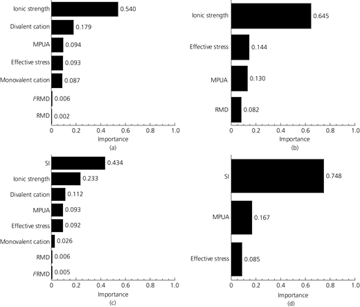
Importance of input parameters on the training data set by regression analysis (XGBoost algorithm): (a) subset 1; (b) subset 2; (c) subset 4; (d) subset 6
Importance of input parameters on the training data set by regression analysis (XGBoost algorithm): (a) subset 1; (b) subset 2; (c) subset 4; (d) subset 6
The ionic strength (I) played a predominant role in subset 1 (Figure 5(a)). Previous studies concluded that the osmotic swelling of Na-B is sensitive to the ionic strength (e.g. >300 mM) in the surrounding environment – that is, osmotic swelling of Na-B can occur in a dilute solution, whereas a solution with high ionic strength can suppress the osmotic swelling of Na-B (Chen et al., 2018; Di Emidio et al., 2015; Jo et al., 2001; Shackelford et al., 2000; Zainab et al., 2021). The hydraulic conductivity is inversely related to the swelling of Na-B – that is, Na-B with a higher swelling in permeant solution can maintain a low hydraulic conductivity (Chen et al., 2018; Guyonnet et al., 2005; Jo et al., 2001, 2005; Katsumi et al., 2008; Kolstad et al., 2004b; Zainab et al., 2021). Divalent cations ranked at second place among all features because the divalent cations in the solution can replace the original sodium in the exchangeable complex of Na-B, resulting in inhibition of the osmotic swelling of Na-B and high hydraulic conductivity (Jo et al., 2001; Kolstad et al., 2004a).
The MPUA and effective stress also affected the hydraulic conductivity of Na-B GCLs, which ranked third and fourth places in subset 1, respectively. Lee et al. (2005) reported that the hydraulic conductivity of Na-B GCLs with an MPUA of 5.1 kg/m2 to 20 mM calcium chloride was 8.8 × 10⁻¹¹ m/s, whereas Na-B GCLs with an MPUA of 4.0 kg/m2 showed a higher hydraulic conductivity (e.g. 2.0 × 10⁻⁸ m/s) under the same testing conditions (Cruz, 2021). Therefore, Na-B GCL with a higher MPUA might have higher chemical compatibility than Na-B GCL with a lower MPUA under the same testing conditions. Increasing the effective confining stress applied on a GCL results in a decrease in hydraulic conductivity (Bradshaw et al., 2016; Li et al., 2021a; Petrov and Rowe, 1997; Petrov et al., 1997). Li et al. (2021a) reported that the hydraulic conductivity of Na-B GCLs permeated with TFGDS-473 leachate (I = 473 mM) decreased from 3.1 × 10⁻⁷ to 2.1 × 10⁻⁹ m/s as the effective confining stress increased from 20 to 500 kPa.
The concentration of monovalent cation was less important in comparison with the divalent cation concentration (e.g. ranked fifth), because monovalent cations were less aggressive in suppressing the swelling of Na-B than divalent cations at the same concentrations. For example, the SI of Na-B was 23.1 ml/2 g in 100 mM sodium chloride, whereas the SI of Na-B in 100 mM calcium chloride was much lower (e.g. 8.6 ml/2 g) (Jo et al., 2001). The impact of RMD (including I2 × RMD) was at least partially offset by the synergy effect – that was, RMD is calculated using divalent cations and monovalent cations. In subset 2, the ionic strength was also the most important factor followed by effective stress, MPUA and RMD (Figure 5(b)). Without considering monovalent and divalent cations, the importance of ionic strength and RMD increased significantly.
The importance of each feature in subset 4 is shown in Figure 5(c). SI was added as an additional feature. As expected, the SI was the predominant factor that contributed to the model. This result was consistent with the literature and practice that swelling of Na-B could be used as a quick index test to predict the serviceability of Na-B GCLs to leachates (Chen et al., 2018; Jo et al., 2001, 2005; Katsumi et al., 2008; Kolstad et al., 2004a; Lee et al., 2005; Zainab et al., 2021). The ranking of other features was mostly consistent with that in subset 1, except for RMD and I2 × RMD. In subset 6, the SI was also ranked at first place, followed by MPUA and effective stress (Figure 5(d)).
Model performance in testing data
The XGBoost model also consistently had the best performance for testing data set (Table 11). The model performance for testing data using the XGBoost method is shown in Table 5. The performance of subsets 3–5 was better than that of subsets 1 and 2 (e.g. lower MSE, MAE and MAAPE and higher RWI and R2). The results illustrated the significant contribution of SI in predicting the hydraulic conductivity of Na-B GCLs. Subsets 6 and 7 showed relatively poor performance due to ignoring the leachate properties as features (e.g. higher MSE, MAE and MAAPE and lower RWI and R2). Similar to the observed patterns in training data, subsets 3 and 4 showed great results. Subset 4 had the best performance in terms of the smallest MSE, MAE and MAAPE and highest RWI and R2, followed by subset 3. In comparison with subset 3, subset 4 consists of one additional feature - I2 × RMD, which reflects that the sensitivity to RMD varies non-linearly with ionic strength (Kolstad et al., 2004a). Subset 6 had better performance than subset 7 (e.g. MSE: 0.776 against 1.113; R2: 0.747 against 0.637), illustrating the importance of MPUA in predicting the hydraulic conductivity of Na-B GCLs. The testing results of the 70:30 ratio exhibit comparable performance (slightly lower) with those of the 80:20 ratio.
Model performance for testing data using regression analysis (XGBoost algorithm)
| Subset | MSE: log2(m/s) | R2 | MAE: log(m/s) | MAAPE | RWI |
|---|---|---|---|---|---|
| 1 | 0.578 | 0.811 | 0.560 | 0.069 | 0.635 |
| 2 | 0.580 | 0.811 | 0.583 | 0.071 | 0.620 |
| 3 | 0.555 | 0.819 | 0.552 | 0.066 | 0.640 |
| 4 | 0.535 | 0.826 | 0.530 | 0.064 | 0.654 |
| 5 | 0.572 | 0.813 | 0.573 | 0.068 | 0.626 |
| 6 | 0.776 | 0.747 | 0.649 | 0.077 | 0.577 |
| 7 | 1.113 | 0.637 | 0.829 | 0.095 | 0.460 |
A comparison of the predicted hydraulic conductivity and the measured hydraulic conductivity of Na-B GCLs (subsets 4 and 6) is plotted in Figure 6. The results showed that subset 4 led to more accurate prediction than subset 6 with a higher R2 (e.g. 0.826 against 0.747). The majority of predicted hydraulic conductivities using subset 4 were within ten times the measured values. In contrast, more data points fell between ten and 100 times using subset 6.
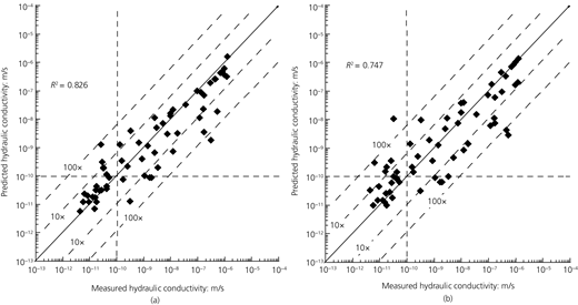
Comparison between the predicted and measured hydraulic conductivities on the testing data set by regression analysis (XGBoost algorithm): (a) subset 4; (b) subset 6
Comparison between the predicted and measured hydraulic conductivities on the testing data set by regression analysis (XGBoost algorithm): (a) subset 4; (b) subset 6
Classification analysis results
Model comparison
In this section, the results of five classification models (logistic regression, XGBoost, SVM, KNN and ANN) are discussed. The accuracy of all five models across all seven subsets are shown in Figure 7. The classification model based on logistic regression showed the worst model performance compared with those with advanced algorithms (e.g. XGBoost, SVM, KNN and ANN). In each subset, the XGBoost method obtained higher accuracy than the other four methods and E (Figure 7(a)). For example, in subset 4, the accuracy of XGBoost was 0.976, which was 14.6, 8.4, 10.5 and 8.4% higher than the accuracy of the logistic regression, SVM, KNN and ANN methods, respectively. The AUC value also supported that the XGBoost method showed the best prediction performance in all seven Subsets, as shown in Figure 7(b). For example, the AUC of subset 4 by the XGBoost method was 0.994, which was 2.8–9.5% higher than those of the other four methods. Herein, the further analysis of classification results thus would be focused on the XGBoost method.
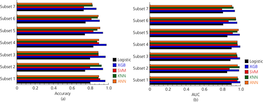
Model performances on training data set by classification analysis using logistic regression, XGBoost, SVM, KNN and ANN: (a) accuracy; (b) AUC
Model performances on training data set by classification analysis using logistic regression, XGBoost, SVM, KNN and ANN: (a) accuracy; (b) AUC
The performance of training models (e.g. seven subsets) using the XGBoost method are shown in Table 6. The accuracy of all seven subsets ranged from 0.866 to 0.976, and the AUCs were between 0.936 and 0.994. Subsets 1 and 2 (leachate properties, effective stress, MPUA) displayed good performance with the accuracy ranging from 0.939 to 0.963 and AUCs ranging from 0.981 to 0.994. By adding an additional feature – the SI – the accuracy of subsets 3–5 increased from 0.939 to 0.976. Subset 6, ignoring leachate properties, yielded lower accuracy (0.919) and AUC (0.962) in comparison with subsets 1–5. Subset 7, further excluding MPUA from subset 6, showed the worst performance among all models, with the lowest accuracy (0.866) and AUC (0.936). The classification model developed in this study did not directly provide hydraulic conductivity prediction, which could be obtained from regression model.
Feature importance analysis
Feature importance in XGBoost models across different subsets was analysed in this section. The importance of features for subsets 1, 2, 4 and 6 is plotted in Figure 8. The ionic strength played a predominant role with importance factors of 0.423, 0.589 and 0.344 in subsets 1, 2 and 4, respectively. This observation was consistent with the previous results that ionic strength significantly affected the hydraulic conductivity of Na-B GCLs (Chen et al., 2018; Jo et al., 2001; Li et al., 2021b; Shackelford et al., 2000; Zainab et al., 2021). Divalent cations ranked second place among all features of leachate properties In subsets 1 and 4, illustrating the adverse effect of divalent cations in solutions on the hydraulic conductivity of Na-B GCLs. In subset 4, SI was added as an additional feature and ranked third place (e.g. 0.176), showing its significant contribution in classifying the hydraulic conductivity. Effective stress and MPUA were ranked after ionic strength and divalent cations (and SI in subset 4). Monovalent cations, RMD and I2 × RMD, however, were the three least important to the classification of Na-B GCLs in subsets 1 and 4.
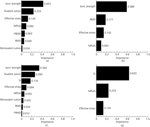
Importance of input parameters on the training data set by classification analysis (XGBoost algorithm): (a) subset 1; (b) subset 2; (c) subset 4; (d) subset 6
Importance of input parameters on the training data set by classification analysis (XGBoost algorithm): (a) subset 1; (b) subset 2; (c) subset 4; (d) subset 6
In subset 2, the ionic strength ranked at first place, followed by RMD. The RMD in subset 2 had a higher contribution in classifying the hydraulic conductivity than the RMD (I2 × RMD) in subsets 1 and 4. The reason that the contribution of RMD (and I2 × RMD) was weakened in subsets 1 and 4 was because of the synergy effect among monovalent cations, divalent cations and RMD – that is, RMD was derived from monovalent and divalent cations (Equation 2).
In subset 6, SI showed a dominating importance factor of 0.633 (Figure 8(d)), which is smaller than that of the corresponding case in regression analysis, 0.748 (Figure 5(d)). In subset 4 with leachate properties, SI became less important, which was ranked at third place after ionic strength and divalent cations, with an importance factor of 0.176 (Figure 8(c)). This observation was different from the regression results of subset 4. In the regression case, SI outperformed other features in subset 4 with an importance factor of 0.434 (Figure 5(c)). These observations indicated that SI played a more important role in predicting than classifying the hydraulic conductivity of Na-B GCLs.
Model performance in testing data
The performance of XGBoost models across all subsets in testing data is summarised in Table 7. The accuracy of all seven subsets ranged from 0.742 to 0.887, with AUCs from 0.825 to 0.931. The model developed from subset 4 was considered the best model since it showed dominating performance in both evaluation metrics. Subsets 1 and 3 displayed great performance, ranked after subset 6. Subsets 1 and 3 had the same accuracy value (0.871), while subset 3 showed a slightly higher AUC value (0.927 against 0.926) than subset 1. Subsets 6 and 7, without considering leachate properties, displayed relatively poor performance, whose accuracy values were below 0.80 (i.e. 0.790 and 0.742, respectively). These results showed that subset 4 provided the best classification of the hydraulic conductivities of Na-B GCLs permeated with saline solution and leachates, which can be an effective method to screen Na-B GCLs in practice.
Conclusions and recommendations
The ML models were used to predict and classify the hydraulic conductivity of Na-B GCLs to leachates. The data set (including 308 observations) was compiled from 22 papers published from 2000 to 2022. Features such as leachate properties (I, RMD, monovalent and divalent cations), MPUA, SI and effective stress were used as input features for the ML models. ML models, including linear regression, logistic regression, XGBoost, SVM, KNN and ANN, were applied and compared in this study. The following conclusions and recommendations were drawn.
- ▪
The XGBoost method outperformed all the other models (linear, Logistic, SVM, KNN and ANN) over all of feature subsets for both regression and classification analyses. The XGBoost method showed a lower MSE value and a higher R2 than other algorithms in regression analysis and higher accuracy and AUC value in classification analysis.
- ▪
Subset 4, including MPUA, effective stress, monovalent and divalent cations, I, RMD, I2 × RMD and SI as features, showed the best performance in testing data, with the lowest MSE and highest R2 in regression analysis and the highest accuracy and AUC value in classification analysis.
- ▪
The XGBoost model using subset 4 as features provided good fitting for both regression and classification tasks. The classification model could be used as a tool to screen qualified Na-B GCLs to specific leachates (e.g. ≤1 × 10⁻¹⁰ m/s), while the regression model could provide good estimation of the hydraulic conductivity of Na-B GCLs.
It is recommended to apply the XGBoost model using subset 4 (e.g. MPUA, σ, monovalent cations, divalent cations, I, RMD, I2 × RMD, SI) for both regression and classification. The regression model can be used to predict the hydraulic conductivity of Na-B GCLs, and the classification model can classify the status of hydraulic conductivity based on the threshold value (e.g. ‘success’ if ≤1 × 10⁻¹⁰ m/s; ‘failure’, otherwise). If leachate properties are unknown, other subsets (e.g. subsets 6 and 7) also can be used by the XGBoost model to obtain a rough estimation of the hydraulic conductivity of Na-B GCLs. Additional laboratory hydraulic conductivity tests should be conducted to validate the results. To evaluate the long-term hydraulic performance of Na-B GCLs, laboratory hydraulic conductivity tests are highly recommended. The cation-exchange process also affected the long-term hydraulic conductivity of Na-B GCLs (Jo et al., 2005). The different rankings of the importance of input parameters were observed in regression and classification analyses, which could not be explained only by statistical analysis in this study. Laboratory experiments should be conducted to investigate the different importance of input parameters observed in regression and classification analyses. In the future, more data are desired to enrich the database to modify and validate the models. A hybrid ML model combining metaheuristic algorithms (e.g. GWO) can be developed and validated to improve further the prediction accuracy and generalisation ability.
Appendix
Tables 8 and 9 show the hyperparameters tuned for regression and classification models, respectively. In each table, the first and second columns list the model and parameter names, respectively, while the third column illustrates the candidate values for grid search. The last column shows the optimal value for the selected model in subset 6 (the subset with best performance).
Parameter settings for regression models
| Model | Parameter name | Candidate values | Optimal value |
|---|---|---|---|
| XGBoost | nrounds | 15, 20, 25, 30, 35 | 30 |
| Eta | 0.3, 0.4, 0.5 | 0.4 | |
| Gamma | 0.2, 0.3, 0.4 | 0.3 | |
| max_depth | 10, 12, 15, 18, 20 | 12 | |
| min_child_weight | 1, 2, 3, 4, 5 | 3 | |
| SVM | Degree | 1, 2, 3, 5 | 2 |
| C | 2, 3, 5, 8, 10 | 3 | |
| Scale | 0.1, 0.3, 0.5 | 0.3 | |
| KNN | K | 2, 3, 4, 5, 6, 7, 8, 9, 10 | 3 |
| ANN | Size | 1, 2, 3, 4, 5, 6, 7, 8 | 6 |
| Decay | 0.0001, 0.001, 0.01, 0.05, 0.1, 0.5 | 0.1 |
Parameter settings for classification models
| Model | Parameter name | Candidate values | Optimal value |
|---|---|---|---|
| XGBoost | nrounds | 3, 5, 7, 10, 15, 20 | 15 |
| Eta | 0.5, 0.7, 0.9, 1 | 1 | |
| Gamma | 0, 0.3, 0.6, 1 | 0.3 | |
| max_depth | 1, 5, 10, 15, 20 | 5 | |
| min_child_weight | 1, 3, 5, 8, 12 | 3 | |
| SVM | Sigma | 0.1, 0.3, 0.5 | 0.3 |
| C | 3, 5, 8, 10 | 8 | |
| KNN | K | 2, 3, 4, 5 | 3 |
| ANN | Size | 5, 10, 15, 20, 25, 30 | 25 |
| Decay | 0.001, 0.005, 0.01, 0.05, 0.1 | 0.05 |
The models are obtained using the R 4.1.2 software with packages caret 6.0, xgboost 1.5.0.2, e1071 1.7 and nnet 7.3.
Table 10 shows the equations for predicting the hydraulic conductivity of Na-B GCLs using the linear regression method based on subsets. Tables 11 and 12 show model performance on training data set and testing data set for regression analysis. The data are provided in the Microsoft Excel file ‘Data-ENGE-2022-181.xlsx’ in the online supplementary material.
Equations for predicting the hydraulic conductivity of Na-B GCLs using the linear regression method based on subsets
| Subset | Empirical equation (linear regression method) |
|---|---|
| 1 | |
| 2 | |
| 3 | |
| 4 | |
| 5 | |
| 6 | |
| 7 |
Model performance of training data using regression analysis
| Subset | MSE: log2(m/s) | R2 | MAE: log(m/s) | MAAPE | RWI | ||||||||||||||||||||
|---|---|---|---|---|---|---|---|---|---|---|---|---|---|---|---|---|---|---|---|---|---|---|---|---|---|
| Linear | XGB | SVM | KNN | ANN | Linear | XGB | SVM | KNN | ANN | Linear | XGB | SVM | KNN | ANN | Linear | XGB | SVM | KNN | ANN | Linear | XGB | SVM | KNN | ANN | |
| 1 | 1.691 | 0.183 | 1.248 | 0.968 | 0.956 | 0.488 | 0.944 | 0.622 | 0.707 | 0.710 | 1.096 | 0.264 | 0.858 | 0.732 | 0.780 | 0.129 | 0.032 | 0.105 | 0.086 | 0.092 | 0.335 | 0.840 | 0.479 | 0.556 | 0.527 |
| 2 | 1.867 | 0.244 | 1.587 | 0.697 | 0.937 | 0.435 | 0.926 | 0.519 | 0.789 | 0.716 | 1.168 | 0.340 | 0.999 | 0.618 | 0.784 | 0.138 | 0.041 | 0.120 | 0.073 | 0.094 | 0.291 | 0.793 | 0.394 | 0.625 | 0.524 |
| 3 | 1.547 | 0.126 | 1.086 | 0.679 | 0.773 | 0.531 | 0.962 | 0.671 | 0.794 | 0.766 | 1.053 | 0.227 | 0.796 | 0.596 | 0.698 | 0.123 | 0.027 | 0.095 | 0.070 | 0.083 | 0.361 | 0.863 | 0.517 | 0.638 | 0.577 |
| 4 | 1.547 | 0.141 | 1.087 | 0.729 | 0.794 | 0.531 | 0.957 | 0.671 | 0.779 | 0.760 | 1.053 | 0.251 | 0.787 | 0.615 | 0.714 | 0.123 | 0.030 | 0.094 | 0.073 | 0.084 | 0.361 | 0.848 | 0.523 | 0.627 | 0.567 |
| 5 | 1.687 | 0.186 | 1.381 | 0.850 | 1.127 | 0.489 | 0.944 | 0.582 | 0.743 | 0.659 | 1.122 | 0.310 | 0.949 | 0.714 | 0.903 | 0.132 | 0.038 | 0.113 | 0.085 | 0.107 | 0.319 | 0.812 | 0.424 | 0.567 | 0.452 |
| 6 | 1.920 | 0.346 | 1.648 | 0.773 | 0.823 | 0.419 | 0.895 | 0.501 | 0.766 | 0.751 | 1.201 | 0.411 | 1.037 | 0.640 | 0.694 | 0.142 | 0.049 | 0.121 | 0.075 | 0.082 | 0.271 | 0.751 | 0.370 | 0.612 | 0.579 |
| 7 | 1.921 | 0.699 | 1.769 | 1.302 | 1.145 | 0.418 | 0.788 | 0.464 | 0.606 | 0.653 | 1.204 | 0.637 | 1.085 | 0.927 | 0.881 | 0.142 | 0.075 | 0.128 | 0.110 | 0.105 | 0.269 | 0.614 | 0.341 | 0.437 | 0.465 |
Model performance of testing data using regression analysis
| Subset | MSE: log2(m/s) | R2 | MAE: log(m/s) | MAAPE | RWI | ||||||||||||||||||||
|---|---|---|---|---|---|---|---|---|---|---|---|---|---|---|---|---|---|---|---|---|---|---|---|---|---|
| Linear | XGB | SVM | KNN | ANN | Linear | XGB | SVM | KNN | ANN | Linear | XGB | SVM | KNN | ANN | Linear | XGB | SVM | KNN | ANN | Linear | XGB | SVM | KNN | ANN | |
| 1 | 1.521 | 0.578 | 1.682 | 1.135 | 1.068 | 0.503 | 0.811 | 0.451 | 0.629 | 0.652 | 1.032 | 0.560 | 1.043 | 0.832 | 0.822 | 0.121 | 0.069 | 0.129 | 0.095 | 0.098 | 0.327 | 0.635 | 0.320 | 0.458 | 0.464 |
| 2 | 1.581 | 0.580 | 1.894 | 1.093 | 1.910 | 0.484 | 0.811 | 0.382 | 0.643 | 0.377 | 1.038 | 0.583 | 1.112 | 0.797 | 1.048 | 0.121 | 0.071 | 0.134 | 0.094 | 0.126 | 0.324 | 0.620 | 0.275 | 0.481 | 0.317 |
| 3 | 1.431 | 0.555 | 1.430 | 1.049 | 0.887 | 0.533 | 0.819 | 0.533 | 0.658 | 0.711 | 1.016 | 0.552 | 0.959 | 0.758 | 0.767 | 0.118 | 0.066 | 0.117 | 0.089 | 0.095 | 0.338 | 0.640 | 0.375 | 0.506 | 0.500 |
| 4 | 1.430 | 0.535 | 1.461 | 1.081 | 0.963 | 0.533 | 0.826 | 0.523 | 0.647 | 0.686 | 1.016 | 0.530 | 0.964 | 0.779 | 0.771 | 0.118 | 0.064 | 0.117 | 0.090 | 0.092 | 0.338 | 0.654 | 0.372 | 0.492 | 0.498 |
| 5 | 1.467 | 0.572 | 1.555 | 1.177 | 1.547 | 0.521 | 0.813 | 0.493 | 0.616 | 0.495 | 1.031 | 0.573 | 0.994 | 0.821 | 1.057 | 0.119 | 0.068 | 0.120 | 0.095 | 0.128 | 0.328 | 0.626 | 0.352 | 0.465 | 0.311 |
| 6 | 1.674 | 0.776 | 1.576 | 1.169 | 1.731 | 0.454 | 0.747 | 0.486 | 0.618 | 0.435 | 1.131 | 0.649 | 1.018 | 0.828 | 1.020 | 0.132 | 0.077 | 0.118 | 0.099 | 0.123 | 0.263 | 0.577 | 0.336 | 0.460 | 0.335 |
| 7 | 1.681 | 1.113 | 1.746 | 1.883 | 1.485 | 0.451 | 0.637 | 0.430 | 0.386 | 0.515 | 1.136 | 0.829 | 1.053 | 1.115 | 1.025 | 0.132 | 0.095 | 0.123 | 0.131 | 0.123 | 0.259 | 0.460 | 0.314 | 0.273 | 0.332 |

