

This paper aims at investigating and highlighting the hydrological benefit of vegetation by way of root water uptake (RWU) in preventing or at least delaying rainfall-induced slope failures in the island of Guam. In particular, the results of field instrumentation and monitoring by way of moisture and suction sensors, laboratory and field testing of geotechnical and hydrological soil properties and rainfall-induced numerical simulations of transient seepage coupled with slope stability analysis are presented. Two case studies, one with a 45° slope and another with a 60° slope, were studied for three different case scenarios. Only one set of vegetation and root reinforcement data was idealised, and the results confirm that matric suction was induced within shallow depths due to RWU helping in providing a buffer, which prevents slope failure during lower-precipitation events. However, this stabilisation effect ceases after saturation during long-duration precipitation. On the other hand, complementary analysis considering the mechanical root reinforcement effect showed that it is a dominating factor in improving the factor of safety even after the slope becomes saturated. In general, native hill slopes with a 45° angle were stable, but the one with a 60° angle failed when a real case rainfall event with climate–vegetation data was applied in this study.
Notation
- af
material parameter related to the air-entry value
- b
constant equal to ln(106) kPa
- Cr
apparent root cohesion
average value of root cohesion
- c′
effective cohesion
- hr
suction at residual water content
- kr(Ψ)
relative hydraulic conductivity function
- ks
saturated hydraulic conductivity
- kx, ky
hydraulic conductivity functions in the x and y directions, respectively
- Lr
width of the vetiver row
- Ls
spacing between vetiver rows
- mf
material parameter function of the residual water content
- mw
slope of the storage curve
- nf
material parameter
- Tr
mobilised tensile stress
- ua
pore air pressure
- uw
pore water pressure
- y
dummy variable of integration representing ln(θ)
- α, n, m
best-fit parameters from Fredlund’s soil water retention curve model
- β
slope angle
- γw
unit weight of water
- Θq
correction factor
- θ′
derivative of volumetric water content with respect to ψ
- θd
angle of shear distortion in the shear zone
- θr
residual volumetric water content
- θw
volumetric water content
- θs
saturated volumetric water content
- φ′
effective frictional angle
- Ψaev
air-entry pressure
- ψ
soil suction
Introduction
Climate-change-related phenomena such as extreme precipitation, prolonged droughts, rising sea level and extreme temperatures and their impact on civil engineering infrastructure have become a universal subject of interest in recent decades. In particular, the effects of extreme precipitation on geotechnical infrastructure such as natural and artificial slopes have been increasingly researched (Alonso et al., 2003; Au, 1998; Chan et al., 2021; Kim et al., 2017; Oh and Lu, 2015; Yang and Vanapalli, 2021). Preservation of coastal ecosystems is of utmost importance for tropical islands, including Guam with limited land, which constantly face the risk of soil depletion due to rainfall-induced slope failures/landslides. Recently, Manibusan et al. (2019) developed a geographic information system–universal soil loss equation-based erosion model and reported an estimated soil loss of 1989.2 (t/km2)/year for the Asan watershed and 1272.59 (t/km2)/year for the Piti watershed in Guam. Eventually, the sedimentation resulting from rainfall-induced shallow slope failures, particularly the one from mountainous terrains of southern Guam, ends up in coastal bays through the network of streams and rivers and pollutes them. This is a leading cause of the damage to the coral life along the coasts of Guam. Thus, the need for finding solutions to prevent hill slope failures in Guam has increased. Also, the geotechnical and hydrological properties of soils from Guam and their application in studying the rainfall-induced slope failure mechanism have been rarely studied. Soil water retention curve (SWRC) tests on undisturbed soil samples, which provide a relationship between moisture and suction for a soil, can indirectly assist in quantifying the water-holding capacity of soil layers, the amount of infiltration within a hill slope and the run-off generated over it. In particular, the SWRC properties of tropical soils in Guam are not available. Hence, efforts are being made by authors to create a data bank of SWRC profiles of soils along hill slopes in Guam.
Vegetation increases the stability of slopes through three governing mechanisms: first, through direct mechanical reinforcement of soil through the roots offering tensile strength; second, by increasing the matric suction of soil through root water uptake (RWU), which is also called transpiration; and third, by dissipating excess pore water pressure (PWP) within the root zone (Indraratna et al., 2006; Jotisankasa and Sirirattanachat, 2017; Khalilnejad et al., 2012; Li et al., 2021; Lobet et al., 2014; Nguyen et al., 2018; Wu, 2013; Zhu and Zhang, 2015). Studies conducted by Feng et al. (2020) revealed that under dry conditions, hydrological effects are more significant. On the other hand, under wet conditions, hydrological effects become insignificant, while mechanical reinforcement dominates in improving slope stability.
It is well known that planting of grasses/trees along steep slopes can be a sustainable bioengineering solution to prevent slope failures. Mahannopkul and Jotisankasa (2019) developed a relationship between root moisture and suction for Chrysopogon zizanioides (vetiver grass) and observed that increasing root suction resulted in decreasing tensile strength. Furthermore, they translated the average root tensile strength into additional root cohesion and incorporated it into the factor of safety (FOS) equation to predict the stability of slopes at different depths for different values of root area ratio (RAR), root suction and soil suction. Interestingly, their studies concluded that the lowest FOS occurred for the hypothetical condition that represented dry vetiver roots in fully saturated soil: a case representing long-term drought following an extreme rainfall event such as a storm. Similarly, Satyanaga and Rahardjo (2019) illustrated through laboratory tests and numerical simulations that the FOS significantly increased for a slope made of old alluvium soil and permeated with Melastoma malabathricum roots. Besides, they concluded that the saturated hydraulic conductivity of alluvium soil permeated with M. malabathricum roots was relatively lower than that of bare soil, which made the plant a great option to be used as a vegetative cover in minimising rainwater infiltration in slopes with angles up to 35°. Ng et al. (2020) conducted field studies to investigate the effects of plant growth and spacing on soil hydrological changes, in particular plant growth-induced changes in percolation, suction and saturated hydraulic conductivity (ks), over a period of more than a year. Through field monitoring, they concluded that closely spaced shrubs preserved most suction during the first 5 months of growth, which was lost after growing for 9 months due to increasing value of Ks. On the other hand, widely spaced shrubs preserved the most suction owing to the least increase in Ks.
Figure 1 shows the hydrologic cycle resulting from water–vegetation–atmospheric interaction, which influences the stability of hill slopes. Soil may exist in saturated, dry and unsaturated conditions. Tropical hill slopes are at high altitudes, and it is unlikely that they will be completely saturated, because the water table is usually at a greater depth. When soil is unsaturated (i.e. above the water table), there exists a negative PWP uw relative to the pore air pressure ua within the soil matrix.
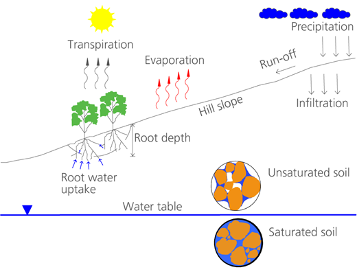
Typical hydrologic cycle between soil–vegetation–atmosphere along a tropical hill slope
Typical hydrologic cycle between soil–vegetation–atmosphere along a tropical hill slope
The numerical difference between pore air and PWPs – that is, (ua − uw) – is also called matric suction. The overall effect of the presence of matric suction is manifested in the form of an increase in shear strength. There exists a highly non-linear relationship between this apparent increase in shear strength with respect to suction (Lu and Likos, 2004; Patil et al., 2017, 2020; Vanapalli et al., 1996). Vanapalli et al. (1996) proposed an equation for modelling the unsaturated shear strength of soil as follows:
where θw is the volumetric water content, θs is the saturated volumetric water content and θr is the residual volumetric water content. If the variation of volumetric water content θw of soil with respect to suction – that is, SWRC – is available, then one can predict the unsaturated shear strength using the Vanapalli et al. (1996) equation. However, this shear strength equation reduces to strength at saturation as the matric suction, and hence, the last term in the preceding equation drops to zero. The preceding equation has been implemented in the Slope/W software (Geoslope, 2018) to conduct slope stability analysis. The FOS was then determined using the Slope/W software of the GeoStudio software package by importing PWP profiles at each time step.
The main objective of this study was to investigate the hydrological effects of roots in improving the stability of tropical hill slopes in southern Guam by way of two mechanisms, mainly RWU and dissipation of excess PWP. There is a lack of similar studies, and to the best knowledge of the authors, this is the first detailed research study on the island of Guam. Although the focus of this paper is on investigating the hydrological benefit of vegetation (i.e. RWU), complementary studies on the other benefit – that is, mechanical root reinforcement – was obtained by using idealised data from some on-site observations and from past literature (Mahannopkul and Jotisankasa, 2019). Two idealised hill slopes – namely, 45 and 60° – with soil profiles similar to that of actual ones at the Ija watershed in southern Guam were considered in performing rainfall-induced transient seepage and coupled slope stability numerical analysis.
The natural tropical environmental setting, which in analysis is represented by input data over a period of 1 year, including climate (i.e. relative humidity, temperature, wind speed, solar radiation and rainfall) and soil properties, was obtained from field instrumentation in the Ija watershed site in southern Guam and laboratory testing. Input data for vegetation were idealised using references from past studies in the literature. The influence of evaporation, evapotranspiration and root reinforcement on the stability of slopes was evaluated through three different case scenarios. The first case considered rainfall on bare ground (slope) without vegetation (only evaporation was considered), which represents a dry and wet season. The second case considered evapotranspiration without precipitation, which represents a long dry season. The third case considered both evapotranspiration and precipitation, which also represents a dry and wet season.
Site location and soil profile
Hill slopes at the Ija watershed located approximately at 13° 15′ 58.104″ latitude, 144° 42′ 59.868″ longitude and altitude of ∼84 m (275.591 feet (ft)) above mean sea level in southern Guam were selected for this study. Field visits revealed that in general, the hill slopes vary in height between 9.144 m (30 ft) and 64.008 m (210 ft) above the general ground surface. The slope height and slope angle varied from several feet to as high as 91.44 m (300 ft) above mean sea level and between 10 and >65°, respectively.
Three-plus yearly site visits by the authors revealed numerous slope failures in the Ija watershed, particularly along hill slopes with the River Ajayan at foothills. It was also observed that the vegetated slopes mostly failed after heavy rainfall events and at locations that had a slope angle exceeding 45°. The topsoil layer supports the roots of the grass or plantation and varies approximately between 0.1524 and 1.2192 m (0.5–4 ft) deep depending on the location. However, the idealised slope is approximately 30 m (98.4252 ft) high, has a 45° slope angle and is made of 0.3048 m (1 ft) of top layer (clayey sand, SC) and 3.048 m (10 ft) of bottom soil (high-plasticity silty clay, CH), followed by 3.048 m (10 ft) of weathered saprolite, which ultimately rests on a sedimentary bedrock of volcanic origin (Figure 2).
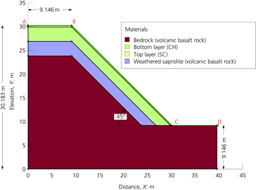
Field observations from previous borings in this watershed indicated that the water table is deep enough and unlikely to rise from a precipitation event into the hill slope, affecting its stability. Transient groundwater flow analyses require an initial condition. Hence, initial conditions for creating a matric suction profile above the water table were imposed by positioning the water table at 3 m elevation on the extreme left boundary and gently sloping to the right boundary with 0.5 m elevation at extreme right (Figure 2). The idea was to make sure that for a 1-year rainfall event, the water table would not rise into the slope, thus avoiding slope failure from a rising water table and thus simulating a real case scenario in this watershed. With this initial position of the water table, the Seep/W software determines the initial negative PWP profile above the water table based on the SWRC of the soil in each layer. After that, the land–climate interaction (LCI) was applied on the ground surface (top surface) of the slope and the PWP changes with time were determined using the Seep/W software.
Material testing and methods
Disturbed and undisturbed soil samples representing each distinct layer within the slope were collected from top, bottom and weathered saprolite layers and were tested in the laboratory for geotechnical and hydrological properties (Table 1). ASTM standards were used for testing of materials – for instance, specific gravity (ASTM, 2002), soil gradation (ASTM (2009) for coarse fraction and ASTM (2007) for fine fraction) and Atterberg’s limit tests (ASTM, 2010) – and finally, the soil was further classified as per the Unified Soil Classification System (USCS).
Soil properties of each layer within the idealised hill slope
| Soil property | Topsoil | Bottom soil | Weathered saprolite | Bedrock |
|---|---|---|---|---|
| Classification (USCS) | Clayey sand (SC) | Silty clay (CH) | — | Volcanic basalt bedrock |
| Unit weight: kN/m3 | 15 | 15.74 | 20 | — |
| Specific gravity | 2.60 | 2.73 | 2.65 | — |
| Porosity | 0.67 | 0.65 | — | — |
| Saturated hydraulic conductivity, ks: m/s | 0.717 × 10⁻⁷ | 0.115 × 10⁻⁸ | 0.706 × 10⁻⁷ | 0.497 × 10⁻⁷ |
| Saturated volumetric water content, θs | 0.669 | 0.649 | 0.40 | 0.50 |
| Effective cohesion, c′: kPa | 5.1 | 8.6 | 15 | — |
| Effective friction angle, φ′: ° | 29.7 | 28.8 | 35 | — |
The percentage proportion of sand:silt:clay in the top layer was 72:18:10, and that in bottom layer was 13:24:63. The liquid limit and plasticity index for of the top layer soil were 42 and 21%, respectively, and those of the bottom layer soil were 85 and 53%, respectively. In addition, SWRC tests were conducted on undisturbed soil samples collected from each of the three layers using Hyprop apparatus and WP4C equipment, both from Meter Group Inc. The SWRC sampling rings, each with a 50 mm height and an 80 mm diameter, were driven into the ground with a hammer using a special sample holder and retrieved with minimal disturbance. Hence, they were undisturbed samples. All Hyprop samples were completely saturated prior to conducting saturated hydraulic conductivity tests followed by SWRC Hyprop–WP4C tests.
Figure 3(a) shows the experimental SWRC data obtained from Hyprop and WP4C equipment for soil samples, which were best fitted with the Fredlund and Xing (1994) model. Also, the saturated hydraulic conductivity (Ks) was obtained through the falling-head method and used to predict the unsaturated hydraulic conductivity with respect to suction through the Fredlund et al. (1994) equation (Figure 3(b)).
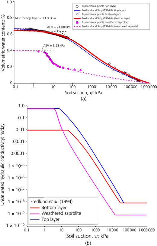
(a) SWRC and (b) unsaturated hydraulic conductivity variations with respect to suction
(a) SWRC and (b) unsaturated hydraulic conductivity variations with respect to suction
The Fredlund and Xing (1994) three-parameter equation was used to fit the experimental data, providing the SWRC over the entire range of suction as follows:
where ψ is the soil suction (kPa), θw is the volumetric water content at soil suction ψ, θs is the saturated volumetric water content, af is a material parameter related to the air-entry value (AEV) of the soil (kPa), nf is a material parameter that is primarily a function of the rate of water extraction from the soil once the AEV has been exceeded, mf is a material parameter that is a function of the residual water content and hr is the suction at the residual water content (kPa). The best-fit parameters – that is, α, n and m – as well as the AEV, saturated volumetric water content (θs) and residual volumetric water content (hr) are presented in Table 2.
SWRC parameters for each soil layer within the idealised hill slope
| Soil layer | SWRC parameters (Fredlund and Xing, 1994) | |||||
|---|---|---|---|---|---|---|
| α: kPa | n | m | AEV: kPa | θs: % | hr: % | |
| Top layer | 146.6129 | 0.5731 | 1.2419 | 13.05 | 0.669 | 0.1013 |
| Bottom layer | 219.6677 | 0.6117 | 1.1479 | 24.08 | 0.649 | 0.1059 |
| Weathered saprolite | 4.4092 | 7.7428 | 0.2133 | 3.68 | 0.400 | 0.2072 |
Moreover, the statistical model proposed by Fredlund et al. (1994) was used to predict the unsaturated hydraulic conductivity for all three soils:
where kr(Ψ) is the relative hydraulic conductivity function; ψ is the suction (kPa); Θq is a correction factor (Mualem, 1986) that takes tortuosity into account; y is a dummy variable of integration representing ln(θ); b = ln(106) kPa; Ψaev is the air-entry pressure; and θ′ is the derivative with respect to ψ. Numerical integration of preceding equation is incorporated through the SVFlux program by SoilVision (2012). Once the soil SWRC and saturated hydraulic conductivity are input, the program calculates the hydraulic conductivity function using the preceding equation.
It should be noted that three undisturbed direct shear test (DST) samples were retrieved by driving steel rings (63.5 mm diameter and 25.4 mm height) from the same depth and nearby locations of each layer from site. The idea was to obtain samples that are almost identical in soil properties such as initial water content, dry unit weight and void ratio. DSTs were conducted on three identical undisturbed soil samples collected from the field under 50, 100 and 150 kPa normal pressures to obtain the consolidated drained shear strength parameters – that is, effective cohesion (c′) and effective friction angle (φ′) – for each layer (Table 1). DST samples were sheared at a slow rate of 0.0043 18 mm/min, which ensured that no excess PWP was developed throughout shearing, thereby maintaining fully drained conditions.
Monthly rainfall data for a 1-year period from the months of April 2020 to March 2021 were collected at 30 min intervals through rain gauge stations installed at the site. These were then converted to the metres per day intensity (Figure 4), which is equivalent to cubic metres per day per square metre, and applied in the LCI tab under the ‘precipitation’ tab for every 0.020833th day (i.e. 30 min) interval using a step function. A tropical depression created a thunderstorm in the month of August 2020, and the rain gauge recorded about 0.233172 m (9.18 inches) of rainfall in 24 h between 27 and 28 August. The highest rainfall of 0.46482 m (18.3 inches) was recorded in the month of August 2020, and the month of November recorded about 0.450088 m (17.72 inch) rainfall. Daily air temperature data for the period of 1 year were obtained from a ZL6 data logger and weather station installed at the Ija site.
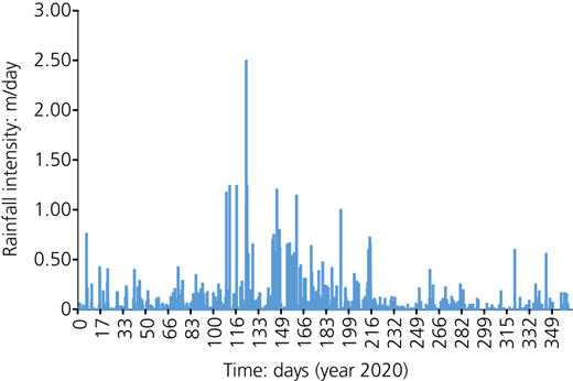
Daily rainfall intensity from data collected over every 30 min interval at the Ija site
Daily rainfall intensity from data collected over every 30 min interval at the Ija site
Field instrumentation
The Ija research station facility owned by the University of Guam and located in the Ija watershed was selected for field instrumentation (Figure 5). Two small and adjacent plots (Figures 5(a) and 5(b)) with gentle slopes of ∼15–20° were instrumented with suction sensors (i.e. Teros 21) and moisture sensors (i.e. Teros 12), both manufactured by Meter Group Inc.
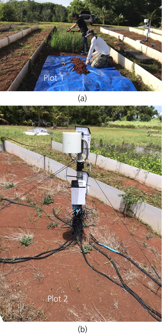
Actual photographs of (a) borehole auguring during field instrumentation of a slope vegetated with young vetiver grass and (b) a rain gauge station with a ZL6 data logger on the bare slope
Actual photographs of (a) borehole auguring during field instrumentation of a slope vegetated with young vetiver grass and (b) a rain gauge station with a ZL6 data logger on the bare slope
Two shallow-depth boreholes were hand augured: the first one on a vegetated slope (first plot) and the second one on a bare slope (second plot). Each borehole was instrumented with a suction sensor at 0.1524 m (0.5 ft) and a moisture sensor at 0.4572 m (1.5 ft). Both boreholes were then carefully backfilled with the soil in the same sequence as it was augured. Each sensor was then connected to a data logger (Figure 5(b)), and approximately 1-year worth data at 30 min interval were collected. The top and bottom layers were profiled from the information obtained from two augured boreholes used for field instrumentation. There were several cut sections available in the watershed that were observed and used to idealise the rest of the soil profile (weathered saprolite and bedrock) at the site.
Analysis of data from field instrumentation
Data retrieved from the data logger in the form of the variation of matric suction with time from Teros 21 (T21) sensors at a depth of 0.1524 m (0.5 ft) on bare and vegetated slopes are shown in Figure 6(a). It should be noted that the topsoil layer – that is, clayey sand (SC) mentioned in numerical analysis – represents the field soil at 0.1524 m (0.5 ft). Comparison of the suction profiles of the two cases at 0.1524 m (0.5 ft) shows that the bare slope retains low suction throughout the year.
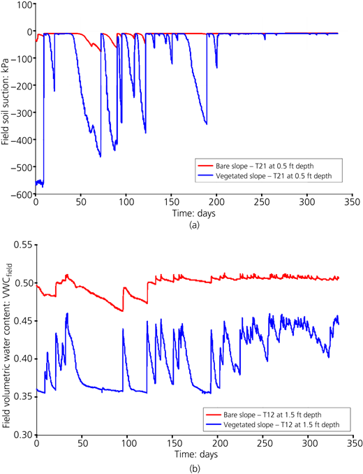
Comparison of (a) field suction profiles and (b) field water content profiles of vegetated and bare slopes
Comparison of (a) field suction profiles and (b) field water content profiles of vegetated and bare slopes
However, the vegetated slope induces appreciable matric suction with the highest value of 465 kPa on approximately the 72nd day (mid of March 2020), which was attributed to the RWU by relatively young vetiver grass at a shallow depth (0.1524 m). Recently, Garg et al. (2020) showed that silty sand causes wilting at much lower suction (around 300 kPa) than clayey loam (around 1600 kPa). However, the root zone depth in this case is about 2 m and into silty clay layer. Interestingly, the maximum value of field suction (i.e. 465 kPa) never reached the general value of the wilting point (∼1500 kPa) even after monitoring for almost one complete year (Figure 6(a)). Thus, it can be said that the soil within slope at the test site (Ija research station) is able to maintain enough water storage to not cause wilting of plants. It is worth mentioning here that the silty clay (CH) – that is, the bottom soil layer used in the previously explained numerical analysis – represents the field soil at 0.4572 m (1.5 ft). Furthermore, the comparison of field moisture profiles at 0.4572 m (1.5 ft) shows that the volumetric water content of the vegetated slope is always less than that of the bare slope, which was expected and can be attributed to the RWU by young vetiver grass at a shallow depth (Figure 6(b)).
Case studies investigating role of vegetation in the stability of hill slopes
Two major case studies were conducted to investigate the role of precipitation and vegetation in the stability of hill slopes through quantification of RWU and mechanical reinforcement. The first one considered a 45° slope angle, and the second one a 60° slope angle. The root reinforcement effect was quantified by assuming typical values of vetiver root morphological characteristics – that is, RAR, root tensile strength from the available literature (Mahannopkul and Jotisankasa, 2019) and some on-site observations related to vetiver plantation. The RAR is the ratio of the sum of the root cross-sectional area to the soil sample plan area and typically varies between 0.2 and 0.8% in vetiver (Mahannopkul and Jotisankasa, 2019). The tensile strength offered by vetiver roots varies with the root diameter and typically ranges between 27.7 and 188 MPa with an average of 117 MPa (Mahannopkul and Jotisankasa, 2019).
Furthermore, the progressive failure of roots was simulated by considering the average mobilised tensile stress offered by roots to be only 40% of their actual tensile strength (Schwarz et al., 2010). The mobilised tensile stress (Tr) developed in roots while being sheared along the failure plane was then translated into apparent root cohesion (Cr) using the Wu et al. (1979) model – that is, Cr = Tr(RAR)(sin θ + cos θ tan φ), where θ is the angle of shear distortion in the shear zone, which is usually taken as 45°, and φ is the soil friction angle. Based on aforementioned typical values, the calculated Cr value in vetiver is 255 kPa. The average value of root cohesion () for the entire slope was then calculated as . In this analysis, based on field observations, Lr = width of the vetiver row = 0.6096 m and Ls = spacing between rows = 1.524 m were assumed. This yields the final average root cohesion value of . The root zone depth in this analysis was 2 m. However, slightly lower values of were used for this analysis. Since, the root density is higher at shallow depths, a relatively higher value of was considered for the top layer, which was 0.3048 m deep. Since the root density decreases with depth, a relatively lower value of was adopted for the rest of the root–soil zone (i.e. for 1.907 m). The assumed values were directly added to the shear strength (Equation 1), and complementary analyses were performed to illustrate the difference in FOS considering (a) a bare ground slope, (b) a vegetated slope considering only RWU and (c) a vegetated slope considering RWU plus root reinforcement. Thus, the differences between the hydrological and mechanical benefits of vegetation were separated for better illustration of their individual contributions along slopes for all case studies that are described in the following sections.
Case study 1: hill slope with a 45° slope angle
Three different case scenarios were investigated. The first was LCI without vegetation, the second was LCI without rainfall and the third was LCI where both vegetation and rainfall effects were considered. Figure 2 shows the geometry and profile of the idealised hill slope.
LCI without vegetation (case 1(a))
In this case, the ground surface was bare – that is, no vegetation – and only evaporation from bare land was considered. The annual (i.e. April 2020–March 2021) precipitation and climate data such as air temperature, relative humidity, wind speed and solar radiation, which were retrieved from the on-site weather station, were applied on the top slope boundary surface (Figures 4 and 7). The sides and bottom had a no-flow boundary condition applied. Thus, there was no flow entering or leaving the system through these nodes.
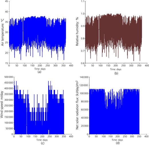
Yearly climate data: (a) air temperature, (b) relative humidity, (c) wind speed and (d) solar radiation for the year 2020 from the weather station
Yearly climate data: (a) air temperature, (b) relative humidity, (c) wind speed and (d) solar radiation for the year 2020 from the weather station
The changes in negative/positive PWPs and land evaporation with respect to time were studied by conducting transient seepage analysis with respect to applied precipitation using a finite-element program by GeoStudio (Geoslope, 2012, 2017) – namely, Seep/W. The input soil properties including the saturated hydraulic conductivity (Table 1), SWRC (Figure 3(a)) and the unsaturated hydraulic conductivity with respect to suction (Figure 3(b)) assist in accurately monitoring the net infiltration into the slope and the resulting surface run-off in response to the precipitation.
The default physical processes in the Seep/W software include pressure- and gravity-driven flow, storage changes due to water compressibility, soil structure compressibility and changes in matric suction with respect to water content. Once the soil properties, SWRC profiles, saturated and unsaturated hydraulic conductivity profiles and boundary conditions are applied, the software calculates the PWP profiles with respect to time for rainfall events. The governing differential equation used in Seep/W finite-element formulation for transient seepage is as follows:
where mw = ∂θ/∂uw = the slope of the storage curve obtained from SWRC; θw is the volumetric water content; H = uw/γw + Y; uw is the pore water pressure; Y is the elevation; γw is the unit weight of water; and kx and ky are the hydraulic conductivity functions in the x and y directions, respectively.
The automatic and robust discretised mesh generation algorithm in the Seep/W software was used to generate the finite-element method mesh for the entire slope model, and it was made of four types of elements – namely, triangular, square, rectangular and trapezoidal elements of different sizes. The Seep/W software then verified and checked the mesh model for any errors and solved the simultaneous water-flow governing equations (Equation 4) for each node thereby, computing the resulting PWP distribution. A separate study regarding the influence of the mesh discretisation on the PWP values was not conducted. Further analysis of the initial PWP profiles existing within the slope starting April 2020 showed that on day 1, the PWP within the slope height is highly negative, varying between −260 and −80 kPa, which represents a dry climate period with the maximum value at the crest portion. However, as the actual rainfall is applied starting the month of April 2020, the PWP within the slope reduces gradually due to infiltration of water during the wet season (July–November) but at a slow rate, resulting in the PWP becoming more positive, causing the matric suction to reduce. On the 217th day, a day after the thunderstorm of November 2020, the value of the PWPs changes to 0 kPa in the top layer and becomes −20 kPa within the bottom layer throughout the crest and sloping portion, resulting in the lowest matric suction (negative PWP) values during the entire year. After the 217th day (i.e. November 2020) – that is, after the wet season – the hill slope does not receive an appreciable amount of rainfall and the slope starts regaining some matric suction as the dry season starts in Guam. Furthermore, the slope regains decent matric suction of about −80 and −60 kPa in top and bottom layers, respectively, by the end of the 365th day.
Plots of infiltration, run-off and evaporation with respect to time show that the entire amount of precipitation that fell on the top climate boundary (ABCD) infiltrated into the slope and there is no run-off generated up to approximately the first 125 days (Figure 8). However, thereafter there is a decent amount of run-off generated (Figure 8(b)). To obtain further insight, the volumetric water content was plotted with respect to depth at different time steps (Figure 9). The saturated volumetric water content (θ) values estimated from the SWRCs of the soil existing in the top and bottom layers were high – namely, θs = 0.669 and 0.649, respectively. This also means that the water storage capacity of the soil in both layers is high. Based on the initial matric suction in soil, the in situ θ at 0 days (around 0.5) is much less than θs (i.e. 0.669 and 0.649, respectively). Hence, all the water from the initial rainfall will infiltrate into the hill slope and there will be no run-off generated, which is evident from Figures 8 and 9. However, after approximately 125 days, the water storage capacity of top and bottom layers is exceeded, resulting in run-off (Figure 8(b)).
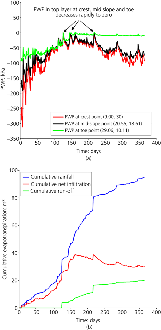
(a) PWPs at a shallow depth of the crest, mid slope and near the toe the of hill slope; (b) cumulative rainfall, net infiltration and run-off over a 1-year period
(a) PWPs at a shallow depth of the crest, mid slope and near the toe the of hill slope; (b) cumulative rainfall, net infiltration and run-off over a 1-year period
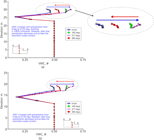
(a) Volumetric water content (VWC) with respect to elevation at the (a) crest and (b) mid slope during different time steps
(a) Volumetric water content (VWC) with respect to elevation at the (a) crest and (b) mid slope during different time steps
Furthermore, the volumetric water content increases with precipitation from the 0th day to the 217th day. However, after that, precipitation decreases and so does the volumetric water content (Figures 9(a) and 9(b)).
LCI with vegetation and no rainfall (case 1(b))
Engineered slopes with vegetation need careful watering, particularly in the dry season to prevent roots from reaching their wilting point. Similarly, vegetation grown over remote natural hill slopes in Guam would also wither during a prolonged dry season. In both cases, the water content and the subsequent stability of slopes would be affected. Hence, this case study aimed to study the effect of vegetation in improving the stability of slopes by way of RWU in the absence of precipitation. In particular, the goal here was to find maximum suction reached in the soil from RWU in the absence of precipitation. Vegetation characteristic data used in LCI for analysis are shown in Figures 10(a)–10(c). The Penman–Wilson method (Wilson et al., 1997), which is a modification of the Penman (1948) equation, is used to calculate the evapotranspiration. It requires wind speed and net radiation data against time data (Figures 10(c) and 10(d)), which were collected from the actual on-site weather station in the Ija watershed in southern Guam. Also, vegetation input data in the LCI boundary condition requires relationships, including leaf area index (LAI) against time, plant moisture limiting function, root depth against time function, normalised root density and soil cover fraction (SCF) against time function, which were idealised from the literature (Feddes et al., 2001; Geoslope, 2017; Prasad et al., 1988).
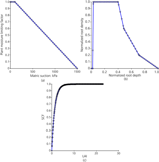
Vegetation data used in analysis: (a) plant moisture limiting factor plotted against matric suction’ (b) normalised root density plotted against normalised root depth; (c) SCF plotted against LAI
Vegetation data used in analysis: (a) plant moisture limiting factor plotted against matric suction’ (b) normalised root density plotted against normalised root depth; (c) SCF plotted against LAI
As shown in Figure 10(a), the root water extraction rate is assumed to be constant and at its maximum initially between suction values of 0–125 kPa and thereafter decreases to zero as it reaches the wilting point – that is, suction of 1500 kPa – due to a reduction in water availability as suggested by Prasad et al. (1988) and Feddes et al. (2001). The root depth changes with time and season and so does the RWU (Feddes et al., 2001). However, for this research, the root depth is kept at a constant value of 2 m. Observations of uprooted vetiver grass in Guam showed that the root density is maximum near the ground surface, and it decreases with depth. Hence, in this analysis, similar variation of the root density is assumed with depth and is represented by the normalised root density against normalised root depth function through Figure 10(b) as suggested in the GeoStudio software package (Geoslope, 2017). The SCF varies from 0 to 1 for bare ground to full coverage conditions, respectively. The LAI is a dimensionless quantity that characterises the plant canopy, and its relationship with ground cover has been idealised as shown in Figure 10(c). It should be noted that in lieu of instruments for measuring the actual vegetation characteristic data, this paper uses the idealised data from past literature and some judgement from authors as discussed earlier. Obviously, it is more generalised and does not strictly represent any particular plant in Guam.
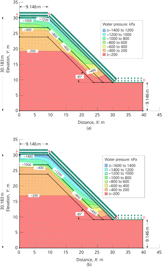
Transient seepage analysis was performed with no rainfall applied to the top boundary. The initial PWP profile was kept same as case (a) for easy comparison. As expected, the magnitude of the negative PWP (i.e. matric suction) became increasingly more negative with respect to time (Figure 11), which also demonstrates the loss of moisture from the soil–root zone on account of the RWU in the absence of rainfall. The PWP was also determined with respect to time at approximately the mid depth of the top layer – that is, shallow depth in the crest (9, 30), mid slope (20.55, 18.61) and toe (29.06, 10.11) regions (Figure 12). Clearly, the PWP was highly and relatively more negative at the crest than at the mid slope and toe portions at a shallow depth (Figure 12).
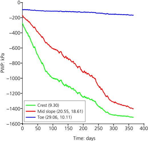
PWP profiles at the crest, mid slope and toe within a shallow depth of the slope
PWP profiles at the crest, mid slope and toe within a shallow depth of the slope
Further insight into analysis of data showed a maximum PWP of −272 kPa at the crest on the 0th day, which becomes equal to −1512 kPa at the end of the 365th day (Figure 12). Interestingly, this value of matric suction is almost equal to the wilting point of the plant, and hence, it is likely that the plant will not survive without watering. Only one climate–vegetation data was idealised and used in this analysis. Different plants will have different RWUs and hence will induce different negative PWPs, which may affect the wilting of plants in the absence of rainfall or artificial watering. Hence, more studies are recommended using data from different plants and seasons.
LCI with vegetation (case 1(c))
In this case, the combined effects of both precipitation and vegetation were considered by applying the LCI over the top surface ABCD. Precipitation data were kept like that of case (a), the vegetation data were similar to that from case (b) and the initial PWP was kept the same as that of cases (a) and (b). Transient seepage analysis revealed that the PWP distribution changes with respect to time, essentially due to infiltration of water from applied precipitation and due to the evapotranspiration phenomenon occurring from the changes in climate and vegetation over time (Figures 13(a) and 13(b)). For the sake of easy comparison with cases 1(a) and 1(b), the PWPs at the 217th and 365th days are shown.
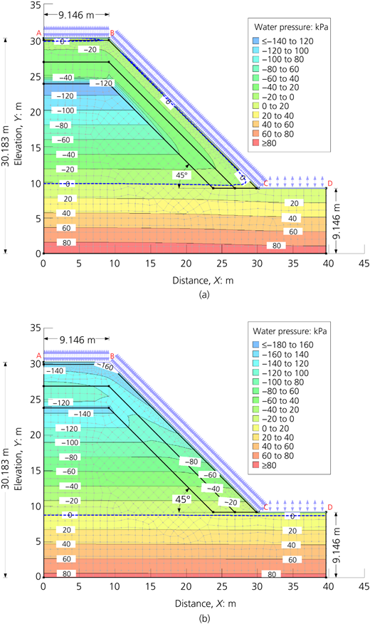
Furthermore, the variations of PWP profiles within shallow depths along the top surface ABCD from all three cases are compared in Figure 14. In all cases, the initial PWP is negative and around the cavitation pressure, which becomes relatively more negative with time in case (b), mainly due to the absence of rainfall and the presence of RWU. On the other hand, the PWP becomes relatively less negative in cases (a) and (c), mainly due to infiltration from rainfall with time. This also shows that the PWP obtained from case (c) lies between those of cases (a) and (b) – that is, PWP case (a) > PWP case (c) > PWP case (b) – which is attributed to the loss of moisture from the root–soil zone due to the RWU in both case (b) and case (c). Analysis of results from case (c) also demonstrates that despite rainfall, the soil can hold a decent amount of matric suction due to RWU, which may likely prolong the slope failure.
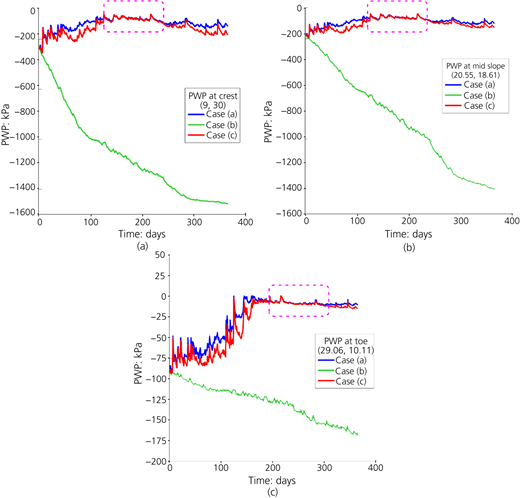
Variation of PWP from all three cases within shallow depths at (a) crest, (b) mid-slope and (c) near-toe portions of the hill slope over a 1-year period
Variation of PWP from all three cases within shallow depths at (a) crest, (b) mid-slope and (c) near-toe portions of the hill slope over a 1-year period
Finally, the transient PWP profiles for all 365 days were imported into the Slope/W software program to perform the coupled slope stability analyses. The classic limit-equilibrium-method-of-slices-based Morgenstern and Price (1965) method analysis, which fully satisfies both ‘force and moment equilibrium’ with the ‘entry and exit’ search technique to identify the critical failure surface with the minimum FOS, was used (Figure 15). The Vanapalli et al. (1996) method was used to model the unsaturated shear strength as a function of soil suction based on the volumetric water content, residual water content and soil water characteristic curve properties for each layer. For case 1(a), the initial FOS using the Morgenstern and Price method is 1.715. The FOS drops down to its minimum (i.e. FOS = 1.20) in two different instances – namely, on the 165th day and 218th day, which are after one of the heavy thunderstorm events (August 2020). These were also the days showing minimum values of matric suction within the slope at the crest and mid slope. Guam is a tropical region with a hot-humid climate, and as such, evapotranspiration rates may play an important role, which were also considered in cases (b) and (c).
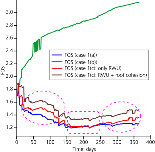
Comparison of FOSs from all three cases illustrating the influence of climate and vegetation on the stability of the hill slope
Comparison of FOSs from all three cases illustrating the influence of climate and vegetation on the stability of the hill slope
In Figure 15, case 1(c): only RWU refers to the inclusion of the RWU effect excluding the root reinforcement effect. Also, for case 1(c): RWU + root cohesion means that both the RWU and root cohesion effects are considered. It is evident from case 1(c): only RWU that in the absence of the root reinforcement effect, the RWU has a more positive effect on stabilising the slope by improving the FOS during low-intensity long-duration rainfall as shown by dashed circles in Figure 15. Such a scenario occurs commonly in Guam during the dry season when it receives less rainfall. However, the slope stability response becomes almost similar during the wet season (near saturation of the root–soil zone), which is marked by storm events such as the ones considered in this study as shown by the dashed rectangle in Figure 15. In fact, FOS recovers rather quickly after the passing of a storm in case of a vegetated slope (i.e. case 1(c): only RWU), as shown in Figure 15. On the other hand, case 1(c): RWU + root cohesion indicates that its FOS is much higher than those of both case 1(a) and case 1(c): only RWU. These findings are in agreement with previous findings in that root cohesion is a dominating factor in bioengineering stabilisation through the vegetation method, even when the root–soil zone is saturated from precipitation. The offered magnitude of root cohesion increases with increasing root tensile strength and root density with depth. Hence, to achieve greater benefit from mechanical root reinforcement, it is essential to choose plants that can grow a deep network of roots and which can exhibit higher tensile strength. Also, during the dry season, the engineered slopes can be more stable if there is no rainfall and the vegetation along slopes are watered carefully to keep the infiltration as low as possible – that is, just enough to keep vegetation healthy (case 1(b)). Moreover, the variation of FOS with time is highly non-linear under the impact of actual rainfall data throughout the year. Case 1(b), case 1(c): only RWU and case 1(c): RWU + root cohesion clearly illustrate that the presence of vegetation does increase the stability of the slope (Figure 15).
Case study 2: hill slope with a 60° slope angle
More than three years of field observations through personal visits by the authors in the Ija watershed indicated that, in general, the hill slopes with an angle greater than 50° had failed. Hence, a slope with a 60° angle was idealised to investigate the effect of increasing inclination on its stability. The thickness of soil layers and their properties were the kept same as those of case study 1.
Transient seepage and coupled slope stability analyses were performed like those explained in case studies 1(a)–1(c). For the sake of easy comparison, the variations of FOS with respect to time are plotted together for cases 2(a)–2(c) in Figure 16. Analysis of the results shows that the FOS drops after the application of rainfall in cases 2(a) and 2(c). However, in case 2(b), the FOS increases continuously and non-linearly in the absence of rainfall while reaching a maximum value of 4.4. This is attributed to the increasing matric suction created through RWU, which results in increasing FOS (case 2(b)).
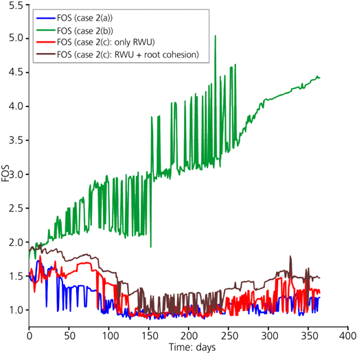
Table 3 summarises the FOS obtained from all different cases for 45 and 60° slopes. Close observation of cases 2(a) and 2(c) in Figure 16 shows that vegetation improves the stability of a 60° hill slope during initial rainfall events (approximately days 25–100). To be precise, the FOSs on the 102nd day were 0.983, 1.382 and 1.566 from case 2(a), case 2(c): only RWU and case 2(c): RWU + root cohesion, respectively. Thus, initially, the presence of vegetation in case 2(c) (both only RWU and RWU + root cohesion) can prevent slope failure (FOS > 1) compared with case 2(a) (non-vegetated slope), which undergoes slope failure (FOS < 1). However, after prolonged rainfall – that is, between approximately days 112–250 – both cases 2(a) and 2(c): only RWU react almost similarly and the hydrological benefit of vegetation through RWU is no longer significant (Figure 16 and Table 3). This is attributed to the fact the soil has become saturated and hence there is no presence of negative PWP, and any matric suction created previously from RWU is lost due to additional rainfall-induced infiltration that keeps the soil saturated. This results in no further increase in shear strength and FOS. On the other hand, the FOS for case 2(c): RWU + root cohesion helps generate a slightly higher FOS compared with the latter two cases. However, both RWU and root cohesion are not enough to prevent slope failure, and thus, beyond 102 days, the 60° vegetated slope is unable to remain stable and eventually fails (Figure 16).
Comparison of FOSs from all three cases
| Slope angle, β: ° | Time: days | FOS | |||
|---|---|---|---|---|---|
| Case (a) | Case (b) | Case (c): only RWU | Case (c): RWU + root cohesion | ||
| 45 | 0 (initial) | 1.715 | 1.871 | 1.728 | 1.883 |
| 52 | 1.404 | 2.522 | 1.481 | 1.594 | |
| 102 | 1.330 | 2.689 | 1.449 | 1.563 | |
| 354 | 1.262 | 3.155 | 1.324 | 1.474 | |
| 60 | 0 (initial) | 1.549 | 1.756 | 1.510 | 1.875 |
| 52 | 0.979 | 2.118 | 1.536 | 1.729 | |
| 102 | 0.983 | 2.164 | 1.382 | 1.566 | |
| 354 | 1.180 | 4.382 | 1.304 | 1.496 | |
Thus, vegetation has a more positive effect in stabilising a 60° hill slope by improving FOS during the initial rainfall event. This is evident from the analysis (Figure 16), which shows that the slope without vegetation fails approximately on the 52nd day (case 2(a)), while the one with vegetation cover takes a longer time to fail (approximately on the 112th day (case 2(c): only RWU)). However, a 60° hill slope for both cases 2(a) and 2(c) reacts similarly during long-duration rainfall events (after day 112) and eventually fails. Hence, it can be concluded that for a 60° hill slope, the vegetation effect is still effective in preventing slope failures during low-intensity and short-duration rainfall events, but this stability mechanism (RWU plus root cohesion) becomes ineffective during prolonged and high-intensity rainfall.
Comparison between field study and numerical simulations
The maximum and minimum values of suction from numerical simulations and that from field monitoring are summarised in Table 4. Field data from a bare land plot and a vegetated plot from a 0.1524 m (0.5 ft) depth are compared with those from numerical simulations at a shallow depth within the top layer at the crest and mid slope from case (a) and case (c), respectively (Figure 17(a)). Clearly, the measured maximum field suction value (−77.3 kPa) was much lower than those from numerical simulations at the crest (−311.6 kPa) and mid slope (−191.2 kPa) for case (a).
Comparison of PWPs from field (∼15–20° slope) and numerical studies (45° slope)
| Field study | Numerical study | |||||
|---|---|---|---|---|---|---|
| Suction value | Bare land slope (0.5 ft depth) | Vegetated slope (0.5 ft depth) | At crest (9 m, 30 m) | At mid slope (20.55 m, 18.61 m) | ||
| Case (a) | Case (c) | Case (a) | Case (c) | |||
| Maximum suction: kPa | −77.3 | — | −311.6 | — | −191.2 | — |
| Minimum suction: kPa | −8.8 | — | 0.96 | — | 0.63 | — |
| Maximum suction: kPa | — | −465 | — | −301.5 | — | −188.6 |
| Minimum suction: kPa | — | −9.69 | — | 0.86 | — | 0.57 |
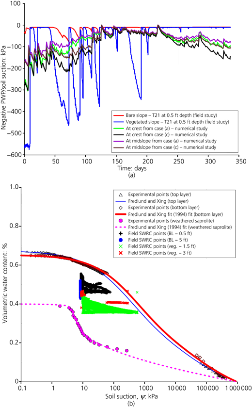
Comparison between (a) suction/negative PWP from numerical simulations at a shallow depth of the crest and mid slope with field measurements from a vegetated and a bare land slope; (b) moisture–suction data from field sensors with lab-based SWRC. BL, bare land
Comparison between (a) suction/negative PWP from numerical simulations at a shallow depth of the crest and mid slope with field measurements from a vegetated and a bare land slope; (b) moisture–suction data from field sensors with lab-based SWRC. BL, bare land
On the other hand, the measured field suction (−465 kPa) was much higher than that from numerical simulations at the crest (−301.5 kPa) and mid slope (−188.6 kPa) for case (c). Interestingly, the minimum value of suction from both bare (−8.8 kPa) and vegetated (−9.69 kPa) field slopes never reached zero suction or positive PWP values. On the other hand, the numerical simulations reveal slightly positive PWPs in cases (a) and (c) the at crest and mid slope. Again, direct comparisons and validations between field and numerical analyses were not possible due to difference in their slope geometry.
The field moisture measured by the T12 sensor at a 0.4572 m (1.5 ft) depth shows a maximum value of 0.513 and a minimum of 0.463 for a bare land slope, while it shows a maximum of 0.460 and a minimum of 0.354 volumetric moisture content for a vegetated slope. Comparison also shows that the measured field volumetric moisture content is always lower than that from simulations.
Furthermore, the field-measured moisture–suction data points are plotted on the laboratory-based SWRC in Figure 17(b). Clearly, both the field moisture and suction values are relatively lower than the lab-based SWRC values. It should be noted that the numerical simulations use the lab-based moisture–suction relationship. Hence, the maximum and minimum values of moisture in Figure 9 are relatively higher than those from the field sensors. This discrepancy is attributed to the soil heterogeneity in the natural slope over which instrumentation was done and fewer SWRC samples tested. Although it is beyond the scope of present study, it is recommended that numerous SWRC samples be collected and the probabilistic analysis approach be used in numerical simulations to incorporate the material heterogeneity to improve the predictions.
Conclusion
Two case studies were presented in this study, one with a 45° slope angle and another with a 60° slope angle. The experimentally obtained soil parameters were used in analysing the stability of an existing slope from the Ija watershed in southern Guam under 1-year precipitation data to perform detailed hydromechanically coupled (i.e. transient seepage coupled slope stability) analysis. The benefits of having vegetation on slopes are compared with those of bare (control soil) through the FOS (dimensionless number) of the slope by way of numerical simulations. Three different case scenarios were considered. The first case scenario included LCI neglecting vegetation to simulate the response of a bare ground slope to antecedent and storm rainfall. A real case, 1-year rainfall data from April 2020 to March 2021, was used for simulations. The second case scenario included LCI without rainfall to investigate the effect of vegetation on engineered slopes (without rainfall). Particularly, the role of transpiration – that is, by way of RWU – and mechanical root reinforcement by way of root cohesion was studied. Results from case scenario 2 suggest that vegetation imposes matric suction within the slope at its maximum and this improves slope stability enormously. This also indicates that during the dry season, engineered slopes can be more stable if there is no rainfall and the vegetation along slopes need to be watered carefully to keep the infiltration as low as possible – that is, just enough to keep vegetation healthy. The third case scenario included LCI to investigate the role of vegetation in stabilisation under year-long precipitation (antecedent and storm rainfall events). This is a natural scenario that is more likely to occur. Results show that RWU tends to reduce moisture in the root zone, thereby increasing matric suction and hence soil shear strength, which ultimately improves resisting forces against sliding. As seen through Figures 14(a)–14(c), the suction in case (c) is always relatively higher than that in case (a) during relatively low-intensity and shorter-duration rainfall – that is, around 75 days – which is indirectly reflected in increasing FOS as indicated in Table 3. It is due to this decent amount of suction held by the top layer in case (c) that the slope stability increases for low-intensity and short-duration rainfall. However, during prolonged rainfall (wet season), this positive effect of stabilisation ceases and vegetated and non-vegetated slopes respond similarly. The effect of mechanical root reinforcement was simulated by using idealised data from some on-site observations and from past literature. Results indicated that root cohesion is the dominant factor in improving the FOS of a 45° slope, and despite a long-duration extreme rainfall event, it considerably improves the stability of the slope.
The second case study was like case study 1, except that the slope angle was 60°. The slope in case study 1 (45° slope) never failed throughout the analysis – that is, its FOS was much greater than 1 – in case of both vegetated and non-vegetated slopes for all case scenarios. This was attributed largely to the greater reduction in the magnitude of rainfall-induced suction and an increase in the magnitude of driving forces around the failure plane owing to the steepness of the 60° slope compared with that of the 45° slope. The analysis with 60° slope angle shows that it fails multiple times both with and without vegetation. Interestingly, it was observed that during the dry season (with low rainfall), the 60° slope remains stable in the presence of vegetation while it fails in the absence of vegetation. However, once the wet season starts (long-duration rainfall), the positive effect of vegetation is lost and vegetated and non-vegetated slopes respond in the same way (i.e. they fail). Thus, it was confirmed that for a 60° slope, the presence of vegetation helps in slope failure during lower-precipitation events but fails to provide stabilisation during long-duration precipitation.
Analysis of data from field instrumentation of a natural slope with and without vegetation located in the same watershed (Ija) with moisture and suction sensors was presented. Results confirm that vegetation induces an appreciably larger magnitude of matric suction within soil–root zone depth, which results from RWU as compared with the bare slope. However, direct comparison of field analysis with numerical analysis was not possible mainly due to difference in slope geometry. Interestingly, the measured field moisture and suction values were found relatively lower than the values obtained from lab-based soil water retention relationship, which was attributed to the material heterogeneity within the natural slope. It is important to mention that only one set of vegetation data was used in quantifying the RWU, and vetiver root-cohesion-related data were obtained from the literature; hence, this study is limited. In the future, it is recommended to conduct slope stability analysis for different soil types and different vegetation data, which could possibly assist in identifying the appropriate vegetation suitable for a watershed in landslide mitigation.





Acknowledgements
This material was supported by the National Sea Grant College Program of the US Department of Commerce, National Oceanic and Atmospheric Administration Award NA18OAR-4170077 (Project R/UOGSG19-2). This material was also supported by the National Science Foundation under Grant OIA-1457769-GEC seed funding year 4 and year 5. The views expressed herein do not necessarily reflect the views of any of these organisations. The authors thank research assistants Giordan Kho, Daniel Mabagos and Edriel Aquino, who are students from the School of Engineering, for their valuable support in conducting laboratory experiments related to this research. Also, the authors thank Dr Golabi from the University of Guam for providing the research area at the Ija research station.

