1-20 of 6339
Follow your search
Access your saved searches in your account
Would you like to receive an alert when new items match your search?
Journal

Fresh perspectives on geoenvironmental engineering.
Journal Articles
Durability mechanisms of MICP-treated granite residual soil under wetting–drying cycles
Available to Purchase
Journal:
Environmental Geotechnics
Environmental Geotechnics 1–16.
Published: 12 June 2026
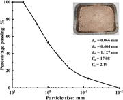
Grain-size distribution curve of granite residual soil A particle size d...
Available to Purchase
in Durability mechanisms of MICP-treated granite residual soil under wetting–drying cycles
> Environmental Geotechnics
Published: 12 June 2026
Figure 1. Grain-size distribution curve of granite residual soil A particle size distribution curve shows percentage passing against particle size in millimetres with soil sample parameters and a soil tray inset. The particle size distribution curve shows percentage passing on the y-axis from ... More about this image found in Grain-size distribution curve of granite residual soil A particle size d...
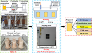
Specimen preparation and experimental procedure A workflow diagram shows...
Available to Purchase
in Durability mechanisms of MICP-treated granite residual soil under wetting–drying cycles
> Environmental Geotechnics
Published: 12 June 2026
Figure 2. Specimen preparation and experimental procedure A workflow diagram shows M I C P specimen preparation, wetting and drying cycles, and subsequent laboratory testing procedures. The workflow diagram illustrates preparation and testing procedures for M I C P-treated soil specimens. On t... More about this image found in Specimen preparation and experimental procedure A workflow diagram shows...
(a) Surface erosion morphology under different W–D cycles and curing times,...
Available to Purchase
in Durability mechanisms of MICP-treated granite residual soil under wetting–drying cycles
> Environmental Geotechnics
Published: 12 June 2026
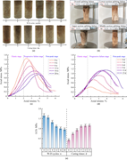
Figure 3. (a) Surface erosion morphology under different W–D cycles and curing times, (b) failure patterns of MICP-treated specimens in unconfined compression tests, (c) stress–strain responses under different numbers of W–D cycles, (d) stress–strain responses under different curing times, and (e)... More about this image found in (a) Surface erosion morphology under different W–D cycles and curing times,...
(a) Failure characteristics of specimens in triaxial shear tests, (b) devia...
Available to Purchase
in Durability mechanisms of MICP-treated granite residual soil under wetting–drying cycles
> Environmental Geotechnics
Published: 12 June 2026
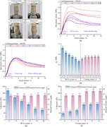
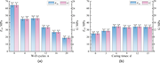
Figure 4. (a) Failure characteristics of specimens in triaxial shear tests, (b) deviatoric stress–strain curves under different numbers of W–D cycles at a confining pressure of 100 kPa, (c) deviatoric stress–strain curves under different curing times at a confining pressure of 100 kPa, (d) peak deviatoric stress (qp) under different W–D cycles and curing times at a confining pressure of 100 kP, (e) evolution of cohesion and internal friction angle under different numbers of W–D cycles, and (f) evolution of cohesion and internal friction angle under different curing times Failure photographs, stress-strain curves, and bar charts compare wetting-drying cycles and curing times under triaxial shear conditions. The multi-panel depicts triaxial shear behaviour of treated soil specimens under different wetting-drying cycles and curing times. Panel a depicts four cylindrical specimen failure modes labelled Overall shear failure, Lower-section shear failure, Upper-section shear failure, and Bulging failure, with corresponding stress differences and confining pressures given in kilopascals and megapascals. Panels b and c depict line graphs of deviatoric stress versus axial strain under a confining pressure of 100 kilopascals for different wetting-drying cycles and curing times. The x-axis represents axial strains in percent, and the y-axis represents deviatoric stress in megapascals. The curves are divided into the elastic stage, the plastic stage, and the strain-softening stage. Panel d depicts grouped bar charts comparing peak deviatoric stress values for wetting-drying cycles and curing times, showing decreasing strength with increasing wetting-drying cycles and increasing strength with longer curing times. Panels e and f depict grouped bar charts comparing cohesion in kilopascals and internal friction angle in degrees for different wetting-drying cycles and curing durations. More about this image found in (a) Failure characteristics of specimens in triaxial shear tests, (b) devia...
(a) Variation in secant modulus and shear modulus under different numbers o...
Available to Purchase
in Durability mechanisms of MICP-treated granite residual soil under wetting–drying cycles
> Environmental Geotechnics
Published: 12 June 2026
Figure 5. (a) Variation in secant modulus and shear modulus under different numbers of W–D cycles, and (b) variation in secant modulus and shear modulus under different curing times Bar charts compare E 50 and G values for different wetting-drying cycles and curing times of treated soil specime... More about this image found in (a) Variation in secant modulus and shear modulus under different numbers o...
(a) XRD patterns of specimens under different numbers of W–D cycles, (b) ...
Available to Purchase
in Durability mechanisms of MICP-treated granite residual soil under wetting–drying cycles
> Environmental Geotechnics
Published: 12 June 2026
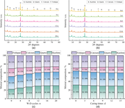
Figure 6. (a) XRD patterns of specimens under different numbers of W–D cycles, (b) XRD patterns of specimens under different curing times, (c) variation in relative mineral content under different numbers of W–D cycles, and (d) variation in relative mineral content under different curing times... More about this image found in (a) XRD patterns of specimens under different numbers of W–D cycles, (b) ...
Pore-scale evolution of MICP-treated granite residual soil under different ...
Available to Purchase
in Durability mechanisms of MICP-treated granite residual soil under wetting–drying cycles
> Environmental Geotechnics
Published: 12 June 2026
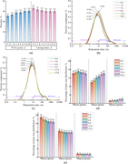
Figure 7. Pore-scale evolution of MICP-treated granite residual soil under different W–D cycles and curing times: (a) variation in total porosity under different W–D cycles and curing times, (b) T2 relaxation spectra for specimens under different numbers of W–D cycles, (c) T2 relaxation spectra for specimens under different curing times, (d) pore-throat size distribution under different numbers of W–D cycles, and (e) pore-throat size distribution under different curing times Porosity charts and pore size distribution curves compare wetting-drying cycles and curing times in treated soil specimens. The multi-panel depicts porosity measurements and pore size distribution analyses for treated soil specimens subjected to varying wetting-drying cycles and curing times. Panel a depicts a bar chart of porosity percentages for wetting-drying cycles and curing times, showing increasing porosity with additional wetting-drying cycles and decreasing porosity with longer curing durations. Panels b and c depict line graphs of porosity component percentage against relaxation time in milliseconds on a logarithmic x-axis for different wetting-drying cycles and curing times. The graphs identify Micro-pores, Meso-pores, and Macro-pores regions. Panels d and e depict grouped bar charts comparing percentages of Micro-pores, Meso-pores, and Macro-pores for different wetting-drying cycles and curing durations. The charts show decreasing Micro-pore percentages and increasing Meso-pore and Macro-pore percentages with increasing wetting-drying cycles, while curing time produces smaller variations in pore distribution. More about this image found in Pore-scale evolution of MICP-treated granite residual soil under different ...
Relationships among mechanical strength, calcium carbonate content, and por...
Available to Purchase
in Durability mechanisms of MICP-treated granite residual soil under wetting–drying cycles
> Environmental Geotechnics
Published: 12 June 2026
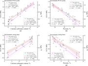
Figure 8. Relationships among mechanical strength, calcium carbonate content, and porosity under different W–D cycles and curing times: (a) variation of UCS and peak deviatoric stress with calcium carbonate content under different numbers of W–D cycles, (b) variation of UCS and peak deviatoric... More about this image found in Relationships among mechanical strength, calcium carbonate content, and por...
SEM images of MICP-treated granite residual soil under different W–D cycle...
Available to Purchase
in Durability mechanisms of MICP-treated granite residual soil under wetting–drying cycles
> Environmental Geotechnics
Published: 12 June 2026
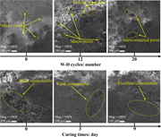
Figure 9. SEM images of MICP-treated granite residual soil under different W–D cycles and curing times Scanning electron microscopy panels show pore structures and cementation changes under wetting-drying cycles and curing times. The six-panel depicts scanning electron microscopy views of tr... More about this image found in SEM images of MICP-treated granite residual soil under different W–D cycle...
Mechanisms governing the deterioration of mechanical properties of MICP-tre...
Available to Purchase
in Durability mechanisms of MICP-treated granite residual soil under wetting–drying cycles
> Environmental Geotechnics
Published: 12 June 2026
Figure 10. Mechanisms governing the deterioration of mechanical properties of MICP-treated granite residual soil under W–D cycles Two sets of sequential soil particle illustrations show calcium carbonate bonding, water flow, and damage to bonded soil structures. The two rows of four sequential... More about this image found in Mechanisms governing the deterioration of mechanical properties of MICP-tre...
FTIR spectra of bentonite, BKC, and 5SBS An F T I R spectrum compares B...
Available to Purchase
in Adsorptive performance of mesoporous silica-modified Bangkok clay as an alternative GCL
> Environmental Geotechnics
Published: 05 June 2026
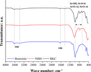
Figure 1. FTIR spectra of bentonite, BKC, and 5SBS An F T I R spectrum compares Bentonite, 5 S B S, and B K C samples with labelled hydroxyl and silicate absorption bands from 4000 to 400 reciprocal centimetre. An F T I R spectrum presents transmittance on the vertical axis and wave number i... More about this image found in FTIR spectra of bentonite, BKC, and 5SBS An F T I R spectrum compares B...
XRD spectra of (a) bentonite and 5SBC and (b) BKC and 5SBS An X-ray d...
Available to Purchase
in Adsorptive performance of mesoporous silica-modified Bangkok clay as an alternative GCL
> Environmental Geotechnics
Published: 05 June 2026
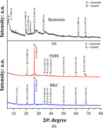
Figure 2. XRD spectra of (a) bentonite and 5SBC and (b) BKC and 5SBS An X-ray diffraction graph compares Bentonite, 5 S B S, and B K C samples with labelled mineral peaks for smectite, kaolinite, and quartz. The figure contains two stacked X-ray diffraction plots with intensity in arbitrar... More about this image found in XRD spectra of (a) bentonite and 5SBC and (b) BKC and 5SBS An X-ray d...
SEM images of (a) bentonite, (b) BKC, and (c) 5SBS Three scanning elect...
Available to Purchase
in Adsorptive performance of mesoporous silica-modified Bangkok clay as an alternative GCL
> Environmental Geotechnics
Published: 05 June 2026
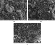
Figure 3. SEM images of (a) bentonite, (b) BKC, and (c) 5SBS Three scanning electron micrographs labelled a, b, and c present layered and clustered particle structures at 10 micrometre scale. The figure contains three scanning electron micrographs arranged with panels a and b at the top and ... More about this image found in SEM images of (a) bentonite, (b) BKC, and (c) 5SBS Three scanning elect...
Pore size distribution of adsorbents A line graph compares pore volume d...
Available to Purchase
in Adsorptive performance of mesoporous silica-modified Bangkok clay as an alternative GCL
> Environmental Geotechnics
Published: 05 June 2026
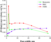
Figure 4. Pore size distribution of adsorbents A line graph compares pore volume distribution versus pore width for Bentonite, B K C, and 5 S B S samples across 0 to 75 nanometres. The graph plots d V divided by d logarithm, w, pore volume in cubic centimetre per gram Ångström against pore wid... More about this image found in Pore size distribution of adsorbents A line graph compares pore volume d...
(a) TGA and (b) DTG of all adsorbents Two thermal analysis graphs co...
Available to Purchase
in Adsorptive performance of mesoporous silica-modified Bangkok clay as an alternative GCL
> Environmental Geotechnics
Published: 05 June 2026
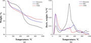
Figure 5. (a) TGA and (b) DTG of all adsorbents Two thermal analysis graphs compare Bentonite, B K C, and 5 S B S samples for weight loss and derivative weight change from 0 to 1000 degree Celsius. The figure contains two side-by-side thermal analysis graphs labelled a and b. Graph A plots... More about this image found in (a) TGA and (b) DTG of all adsorbents Two thermal analysis graphs co...
Pseudo-second-order model of (a) Cu( II ), (b) Zn( II ), and (c) Cd ( II ) ...
Available to Purchase
in Adsorptive performance of mesoporous silica-modified Bangkok clay as an alternative GCL
> Environmental Geotechnics
Published: 05 June 2026
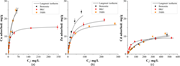
Figure 6. Pseudo-second-order model of (a) Cu( II ), (b) Zn( II ), and (c) Cd ( II ) onto the bentonite, BKC, and 5SBS, non-linear plot at initial metal concentration 200 mg/L, dosage 0.5 g, and pH 5 Three adsorption isotherm graphs compare copper, zinc, and cadmium adsorption by Bentonite, B K... More about this image found in Pseudo-second-order model of (a) Cu( II ), (b) Zn( II ), and (c) Cd ( II ) ...
Adsorption isotherms of metal ions (non-linear plot), (a) Cu ( II ), (b) Zn...
Available to Purchase
in Adsorptive performance of mesoporous silica-modified Bangkok clay as an alternative GCL
> Environmental Geotechnics
Published: 05 June 2026
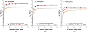
Figure 7. Adsorption isotherms of metal ions (non-linear plot), (a) Cu ( II ), (b) Zn ( II ), and (c) Cd ( II ) onto the bentonite, BKC, and 5SBS surface, contact time 80 min, dosage 0.5 g, and pH 5 Three adsorption kinetics plots compare copper, zinc, and cadmium uptake over contact time for B... More about this image found in Adsorption isotherms of metal ions (non-linear plot), (a) Cu ( II ), (b) Zn...
Adsorption mechanism of SBA-15 modified 1:1 clay A diagram illustrating ...
Available to Purchase
in Adsorptive performance of mesoporous silica-modified Bangkok clay as an alternative GCL
> Environmental Geotechnics
Published: 05 June 2026
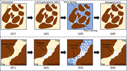
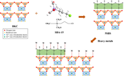
Scheme 1 Adsorption mechanism of SBA-15 modified 1:1 clay A diagram illustrating the synthesis of SBA-15 from BKC, showing molecular structures and ionic interactions involved, including elements contributing to heavy metal removal. More about this image found in Adsorption mechanism of SBA-15 modified 1:1 clay A diagram illustrating ...
