Income and density spillover effects in German land prices

This paper examines the role of agglomeration economies – proxied by median income and population density, in shaping the spatial patterns of land prices across 378 German counties from 2014 to 2018 ^[1]. While the spatial interaction of housing prices has been well-documented in regional science, the contribution of land price spillovers, particularly as distinct from housing structures, remains under-explored. Our paper addresses this gap by focusing explicitly on land prices as both a dependent variable and a spatial transmission channel for housing market dynamics.

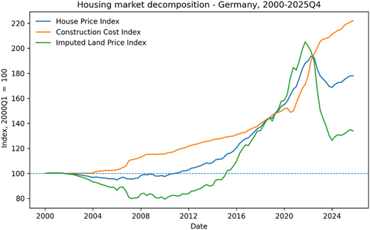
The motivation for focusing on land prices is twofold. First, an emerging literature (e.g. Davis et al., 2021), based on earlier work of Davis and Heathcote (2007), Albouy et al. (2018), Ahlfeldt and McMillen (2020) and Knoll et al. (2017) highlights that rising house prices in developed economies are increasingly driven by the appreciation of land values rather than construction costs. For exposition purposes, Figure 1, which plots the quarterly time series for housing prices, imputed land prices and construction cost indexes for Germany, from 2000 to 2025: Q4 shows the increasing importance of land price development for housing markets, in terms of volatility and movements.

Second, recent evidence from Germany, suggests that the county-level land values are more volatile than housing structures and explain a growing share of housing wealth - underscoring their central role in regional real estate cycles ^[2].

Despite the aforementioned results, most spatial econometric studies in housing economics continue to focus on price spillovers at the level of housing transactions (e.g. Fingleton, 2008; Baltagi et al., 2014; Pijnenburg, 2017), neglecting the composition of these prices into land and structure components. Moreover, while the literature on agglomeration economies (e.g. Ciccone and Hall, 1996; Ciccone, 2002; Glaeser and Gottlieb, 2009) shows that density and productivity shape regional development, little is known about how these forces operate through spatial land price mechanisms.

We contribute to this literature by explicitly modeling income and density induced spatial spillovers in land prices using a spatial panel framework. Our main empirical model of interest is the Spatial Durbin Model (SDM) ^[3], which allows for both endogenous spatial dependence in the dependent variable (prices) and exogenous interactions in agglomeration-related covariates (e.g. median income, population density) ^[4]. Our analysis pursues three core objectives. First, we quantify the direct and indirect effects of county-level agglomeration variables on land prices. Second, we evaluate the extent to which spillovers in land prices contribute to clustering patterns in major German cities and their suburban counties. Third, we assess whether these effects differ by land type - comparing residential land with vacant land designated for development.

We find that spatial agglomeration effects, especially in income and density, exert significant local and neighboring effects on land prices. Specifically, a 1% increase in median income leads to a 1.94% increase in local land prices and an additional 0.71% increase in neighboring counties. Similarly, a 1% increase in population density raises land prices by approximately 2–3% locally and 1–2% indirectly. These effects exhibit greater intensity in suburban counties adjacent to large metropolitan areas. Finally, the effects are more pronounced for residential land than vacant land, consistent with the idea that realized use and regulatory constraints magnify spatial externalities in housing markets.

In doing so, this paper provides a link between the literature on spatial housing dynamics, agglomeration variables and land valuation. Our findings suggest that policy interventions targeting housing affordability or regional price disparities should account not only for housing demand and supply but also for the spatial diffusion of land price shocks, especially in high-productivity regions experiencing density-driven growth. Moreover, the results highlight the importance of regional coordination in housing, land use and infrastructure policies, as changes in economic activity and population density in one county generate significant spillover effects on neighboring land markets. The findings, thus, suggest that housing affordability and land-use challenges should be addressed at a regional scale rather than solely within individual jurisdictions.

For investors, the results indicate that land values are influenced not only by local fundamentals but also by economic developments in surrounding regions. Consequently, investment opportunities may arise in counties that benefit from growth spillovers originating in nearby metropolitan areas, particularly where agglomeration forces remain strong.

This paper builds on and integrates three strands of research: spatial spillovers in housing markets, the role of agglomeration economies in regional price formation and the growing influence of land values in housing wealth.

A large body of work has established the presence of spatial dependence in house prices across different levels of geographic aggregation (e.g. Dubin, 1988; Can, 1990, 1992; Fingleton, 2008). Most empirical models adopt spatial autoregressive specifications, such as the spatial autoregressive (SAR) model or SDM, to capture endogenous interactions among neighboring housing markets (e.g. Baltagi et al., 2014, Brady, 2014; Gong et al., 2020). These models have been applied to cities and counties in the USA, the UK, Germany and China to study price diffusion, displacement effects and yardstick competition.

In parallel, the agglomeration literature has emphasized how density and productivity shape regional outcomes. Ciccone and Hall (1996) and Ciccone (2002) provide foundational evidence for the productivity-density relationship in the USA and Europe, respectively. Glaeser and Gottlieb (2009) further show that urban productivity and amenities drive both firm clustering and housing demand. However, few studies have examined how these agglomeration forces propagate spatially through land values, particularly in European housing markets.

A third strand has emphasized the centrality of land in explaining variations in house prices. Davis and Heathcote (2007), Albouy et al. (2018) and Davis et al. (2021) show that land values, not construction (structure) costs, account for most of the price growth in the US housing markets over time. Recent studies by Braun and Lee (2021) and Knoll et al. (2017) for Germany confirm similar trends: rising land shares are a dominant factor in urban housing appreciation, particularly in high-density regions.

Our paper advances this literature by explicitly analyzing land prices, not just house prices, as both an outcome and a spatial mechanism. We apply spatial econometric techniques not only to capture interactions in housing markets but also to decompose the spatial effects between local agglomeration forces and regional spillovers in land prices. In doing so, we offer a more complete account of how urban and suburban housing markets respond to localized productivity and density shocks, and how these effects propagate across space.

The main empirical interest lies in the spatial interaction patterns of land prices, both of endogenous and exogenous, and the clustering patterns in house prices that can contribute to spatial variations in land prices. Rather than presenting spatial lag models for the empirical analysis, as lags can be easily added, we present a simple reduced form of the spatial housing market that captures variables affecting supply and demand functions.

As in Fingleton and Le Gallo (2008), consider an economy with n counties. In this economy, the determination process of house prices within a region I may not depend only on the demand and supply factors of that region but also on those of regions within commuting distance from county i. Consequently, we assume that demand for real estate (q_i) reacts to changes in income (w_i) of both region i and surrounding regions to reflect the travel-to-work patterns that require workers to cross county borders. Moreover, we assume that demand for real estate depends on natural attributes of a county (E_i) such as green coverage as well as two types of externalities: 1) local externalities formed by agglomeration economies (l_i) and 2) network externalities from cross-county connections (Wl_i, where W is a spatial weighting matrix). A prime example of agglomeration economies is that higher population density counties can increase the likelihood of enjoyable social contacts and meeting like-minded peers, especially attracting young single people. Also, so-called higher-order amenities, such as opera and expensive restaurants that require substantial economies of scale of economies to be sustained, can mostly be found in higher population density places. We also include the size of land (Combes et al., 2010) and median income as well as labor productivity as a robustness check (Ciccone and Hall, 1996; Combes and Gobillon, 2015) to measure the agglomeration effect.

One can further link the local externality to its agglomeration level in economic activities. Mechanisms that support this connection are, for example, a shared and larger labor pool that improves firm-worker matching and knowledge spillovers through shared information during face-to-face meetings (Glaeser et al., 2001; Gong et al., 2020; O'sullivan, 2007). Switching from the single county to a network of counties ^[5], the previously mentioned connection can cause the same benefits resulting from agglomeration economies within such a network. For example, higher-order amenities can be used by people from less densely populated nearby counties to complement their shopping and entertainment facilities. But these amenities also need to be demanded by those people in order to support and maintain the higher population density counties' functionality and local externalities (Gong et al., 2020; Meijers et al., 2016; Meijers and Burger, 2017) ^[6]. Finally, while demand in region i is assumed to negatively depend on the region's house price p_i, this reduced demand spills over to neighboring regions (displaced demand effect: $ãΣi≠jnWijpj$ _ijp_j). Consequently, the demand function for housing is ^[7].

where W_ij spatially links counties with each other. ω_i is the error term that contains other unmodelled demand factors.

The corresponding supply function for housing takes the following form

where _ η_i is the unobserved supply error term. The supply of housing is assumed to increase with the price level of housing in region i. High real estate prices attract real estate developers and it may be more likely that homeowners are willing to offer their properties for sale. However, this also means that high property prices in neighboring counties “steal” away the supply of housing from region i (displaced supply effect: $bΣi≠jnWijpj$⁠). As in Gong et al. (2020), supply is assumed to depend on the restrictiveness of housing supply, H_i.

Rewriting the supply function by solving for p_i, we have

Substituting for q_i yields

Simplifying the equation further gives the empirical form that includes spatial effects as follows:

where u_i = c₁ω_i + ν_i.

Since the focus is on land prices, we modify Equation (1) by including construction costs. As Davis and Heathcote (2007), Davis and Palumbo (2008) and Glaeser et al. (2006) argue that the determination of house price is more complex in the sense that the costs of new construction consist of the cost of putting up the structure in addition to any geographical or regulatory barriers to housing supply. While the former can be assumed to be supplied highly elastically, the latter can cause housing supply to be highly inelastic depending on the location. Following the residual approach in Braun and Lee (2021) ^[8], we decompose house value into a physical cost of construction and the land value. Therefore, from the housing supply perspective, the price of housing will be determined by the cost of new construction, defined above as the sum of construction cost and land value, in places where demand is sufficiently large to justify new construction. Incorporating this decomposition into Equation A.1, the land value is defined as:

where lp_i is the land value per m² in county i, cc_i is a county-specific construction cost factor that measures the effect of county-specific construction costs on land value.

We are interested in two types of spatial spillover effects on land prices: exogenous interaction effects among the explanatory variables and endogenous interaction effects within the dependent variable. Our empirical framework is, thus, based on regional housing markets, agglomeration and land economies.

As in Anselin (1988) and LeSage and Pace (2009), we use one specification, the SDM, shown in Equation (2), to accommodate a vast number of applied situations. It includes a spatial lag of the dependent variable (⁠$ln(P)$⁠) as well as agglomeration variables in (⁠$X$⁠):

where, $Pn×1$ is the vector of land prices, $Xn×r$ incorporates the county-specific characteristics and agglomeration economies and $Wln×r$ represents the network (spatial) externalities. In the empirical analysis, we use the same weight matrix for $Mn×n$ and $Wn×n$⁠. W and M are the spatial weight matrices that define how counties are spatially connected. For example, matrix W allows for local externalities l to spill over between spatially linked counties and hence spillover effects can be modeled as Wl.

In addition to Equation (2), for comparison purposes, we also estimate three other models. We first start with a panel fixed effects (FE) model (no spatial effects) (⁠$ρ=θ1×r=0)$⁠, and then add two other spatial lagged models, namely the spatial autoregressive model (SAR: $θ=0)$ and the spatial lag of X model (SLX: $ρ=0)$ ^[9].

We focus on the SDM as the main model of interest as the likelihood of displacement effects in land prices causing cross-county spillovers being present in the process of land price determination is pretty high. For example, high land prices in one region cause demand for housing to decrease. However, this demand is likely to be displaced to nearby regions. Another mechanism that can explain this type of spillover effect is “yardstick competition”. For example, house sellers and buyers might take into account price signals from house price transactions in a neighboring county, spatially linking house prices with each other (Brady, 2014; Gong et al., 2020) ^[10].

To identify these spillover effects, we report both direct and indirect spatial effects, where the direct effect represents the effect of a change in a county-specific variable on that county’s land value. The indirect effect represents the cross-county spillovers where a change in a county-specific variable affects the land values of other counties ^[11].

We use the annual (2014–2018) land value per square meter of lot size estimates for German counties and county-free cities from Braun and Lee (2021) as a measure of residential land price. Since one of the main focuses of this paper rests on land prices, the data from Braun and Lee (2021) are briefly summarized here. They estimate the changes in the value and price of residential land for the 379 German counties (“Landkreise”) from 2014 to 2018 by combining data from several publicly available sources for academic researchers. For example, the raw initial total Immoscout dataset consists of 292,583 observations, which are classified as new single- and double-family houses between 2014 and 2018. After sorting out the missing data/information on these 292,583 observations, Braun and Lee (2021) use 42,647 listings of new single - and double-family houses over 379 German counties. Using the 42,647 dataset along with the construction costs that were estimated using the cost information from the German Chambers of Architects association (BKI, n.d., which stands for Baukosteninformationszentrum Deutscher Architektenkammern), a database of 1,895 for the cost of housing structures and residential land values at the county level is built for 2014 to 2018. The framework of the approach used is that of Davis and Heathcote (2007), who decompose house value into the value of the structure and land value on the aggregate level for the USA. Some of the results from Braun and Lee (2021) lend support to this paper’s spatial analysis. For example, residential land prices have become relatively more expensive in most German counties. Moreover, the counties around urban centers such as Munich, Stuttgart, Berlin, Hamburg, Dresden and the Ruhr area cities experienced the highest land price increases. However, we also note that, in general, an upward shift in home values, land values and residential land share occurred in almost every state.

For our dataset, we control for several county-level characteristics in different model specifications. First, we use the following variables to measure the agglomeration economies of each county that are known to generate local and network externalities: the counties' land area in $km2$⁠, its median income and population density (Gong et al., 2020). The latter is calculated by dividing the county's population by its land area in $km2$ in a given year. That is, population density is equal to 100 in a county with 100 individuals per $km2$ ^[12]. Second, we include county-specific land and economic characteristics in different model specifications. As an indicator of the environmental amenities of a city, we include the green residential area that is used for recreational purposes divided by a county's land area in $km2$ (green coverage). We measure the amenities of a county in terms of history and culture with the number of available accommodation facilities in that county (e.g. hotels, etc.). Moreover, we include the arable land per $km2$ of land area to measure the restrictiveness of housing supply (Gyourko et al., 2013; Gong et al., 2020). Finally, we use the construction cost, income and unemployment rate as measures for a county's economic situation as control variables. The data and sources are described in detail in the Appendix in Table A.1. Descriptive statistics are provided in Table 1.

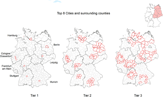
We focus on the first-order contiguity matrix ^[13] estimation for land prices as our spatial regressions. We estimate the models outlined in Section 3 for a total of 378 counties, 314 counties in the old Federal States, 64 counties in the new Federal States and the Big 7 German cities, including their surrounding counties. For expositional purposes, we present Figure 2, which shows the counties assigned to each Tier and Table 2, which presents the number of total counties within Tiers 1–3 ^[14].

Our non-spatial and spatial regression results for German land prices from 2014–2018 are displayed in Table 3. Table 4 compares the SDM results for West – former East Germany and the Big 7 agglomerations.

We begin by presenting the results of the non-spatial baseline model, estimated using FE, as shown in Column (1) of Table 3 ^[15]. With the exception of open accommodation facilities and housing starts, all control variables are statistically significant at the $1%$ or $5%$ level and display the expected signs. An exception is the coefficient on green coverage, which appears with an unexpected sign. While green coverage is typically interpreted as a proxy for local amenities, implying a positive association with land values, it may alternatively reflect constraints on available land for development, which could exert downward pressure on land prices. Similarly, while one might expect the unemployment rate to negatively influence land prices due to its role as an indicator of adverse economic conditions, higher unemployment may be observed in larger urban areas with more dynamic labor markets and higher transitional employment. Cities with higher median income and population density tend to exhibit higher land values, holding other factors constant. In addition to these agglomeration variables, land area per km $2$ – another measure of economic density – shows a statistically significant positive effect on land prices, as reported in Table 3. The FE model yields the following marginal effects: a $1%$ increase in population density raises land values per m $2$ by $2.69%$⁠, ceteris paribus. A $1%$ increase in land area per km $2$ leads to a $4.22%$ increase in land values. In contrast, a $1%$ increase in arable land per capita results in a $0.44%$ decrease in land prices per m $2$⁠, indicating that a more elastic housing supply is associated with lower land values ^[16].

Despite the SDM model being the main model of interest, we also present two other types of spillover effects. First, agglomeration effects are discussed in light of the SLX model, followed by endogenous spillover effects in SAR model.

Our SLX results, reported in Column (2) of Table 3, provide empirical evidence for both local agglomeration effects and network externalities. The coefficient on the spatial lag of population density is positive and statistically significant, indicating that a $1%$ increase in the population density of a neighboring county raises house prices in the county of interest by approximately $0.30%$⁠, ceteris paribus. Similarly, the spatial lag of the log of median income is also positive and significant, further supporting the presence of externalities across regional borders.

Notably, the direct agglomeration variable effects in the SLX model are smaller than those estimated in the FE specification shown in Table 3. Specifically, the coefficients for median income and population density decline by $0.59$ and $0.83,$ respectively, suggesting that part of the effect captured in the non-spatial model may actually reflect spatial interactions.

Moreover, the magnitude of other explanatory variables also changes relative to the non-spatial specification, underscoring the importance of accounting for spatial dependence in model estimation. While the SLX model captures statistically significant spatial lags, the observed spatial dependence may not exclusively stem from externalities in agglomeration variables. Instead, it may also reflect pure spatial spillovers in land values themselves. That is, if spatial dependence is still present after accounting for network externalities, it can be attributed to pure land value spillovers or common shocks. Consequently, if pure land value spillovers cause the remaining spatial dependence, the SDM would be a more valid specification. To disentangle these mechanisms, we compare the SLX results with those from the SAR and SDM models below.

Columns (3) and (4) in Table 3 show the quasi-maximum likelihood estimation (QMLE) estimates of the SAR and the SDM models for the first order contiguity matrix. The estimated coefficient (0.07 for both SAR and SDM) on $Wlt$ for land value, which is statistically different from zero on the 1% significance level in both columns (3) and (4), supports pure land value spillovers.

Compared to FE, most coefficients in the SAR and SDM are robust in terms of size and significance level. As discussed in Section 3, the interpretation of the spatial spillover coefficients for population density and median income may be misleading in the SDM as there might be some other network effects that are present. Compared to columns (2) and (3), we find the SDM to be slightly superior ^[17].

We apply the partial derivative approach outlined in the previous section to compute the direct and indirect spatial effects reported in Table 3. The results provide evidence for both types of effects with respect to population density and median income: these variables influence land values not only within a county but also in neighboring counties across all spatial model specifications in Columns (2)–(4) ^[18].

For instance, in the SLX model, a $1%$ increase in population density in neighboring counties leads to a $0.30%$ increase in land values in the local county, holding other factors constant. The total effect (i.e. the sum of direct and indirect effects) of a $1%$ increase in population density yields an approximately estimated $2to3%$ increase in land values. The total spatial effect for the SDM, on the other hand, is greater than those of both the SLX and SAR models. Specifically, a 1% increase in median income leads to a 1.5–2.5% increase in local land prices and an additional 0.5–0.9% increase in neighboring counties. Similarly, a 1% increase in population density raises land prices by approximately 2–3% locally and 1.5–1.9% indirectly.

Moreover, the direct effects of population density and median income are notably larger in the non-spatial fixed-effects model compared to the spatial models. This discrepancy suggests that omitting spatial interaction terms may result in upward-biased estimates in the non-spatial specification. Since we find statistically significant spillovers in both median income and population density across all three spatial models, the presence of spatial dependence is robust.

The strength of spillover effects varies across model types. Cross-county spillovers for population density are markedly larger in the SAR and SDM models than in the SLX model, indicating that pure spatial interaction effects, beyond network externalities, play an important role in land price determination. Interestingly, the indirect effects in the SDM are smaller than in the SAR model, which implies that spatial dependence in land values may be driven more by direct price spillovers than by agglomeration-related interactions.

Taken together, the results across all models indicate that spatial dependence in land values stems not only from network agglomeration spillovers but also from direct land value spillover mechanisms. This highlights the dual nature of spatial interdependence in regional land markets ^[19].

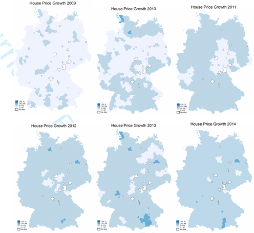
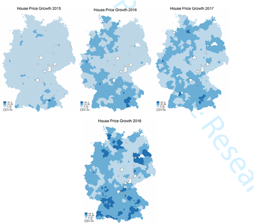
Figure 3 shows the growth in house prices from 2008 to 2018 in German counties. If we informally define a booming housing market as one in which annual growth in house prices is more than 5%, the two darkest blue tones reflect the spread of booming housing markets throughout West German counties and, especially, around large German agglomerations and their neighboring counties ^[20]. Figure 3 informally suggests that the timing of regional housing booms was spatially correlated with and around large agglomerations and West German counties. This descriptive finding could lead to two stylized facts: First, agglomeration and spatial spillover effects might be larger in those regions. Second, booms and, hence, the largest growth in house and land prices are found in counties with previously high levels of house prices, labor productivity and population density. For this reason, this section discusses the SDM estimation results for 314 counties in the old Federal States, 64 counties in the new Federal States and the Big 7 German cities, including their surrounding counties.

Table 4 presents two central findings. First, we observe clear evidence of direct median income effects on land values in West German counties, whereas no such effect is detectable in East Germany. Conversely, the direct population density effect on land values is more pronounced in East German counties than in their West German counterparts. This pattern is further confirmed by results from the Top 7 metropolitan areas. West German cities exhibit a positive direct effect of median income on land values, while such effects are absent in East German cities, including Berlin ^[21] and Leipzig. With the exception of Berlin, Frankfurt and Munich, we find no significant direct agglomeration effects of population density on land values across the Top 7 cities. The estimated effects for Berlin are likely influenced by its proximity to surrounding East German counties.

Second, the evidence for network externalities (indirect effect) is not robust in all areas. We find only modest but statistically significant empirical support for positive spillover effects of median income on neighboring counties' land values in West Germany. These income-based spillover effects are also present in three out of five West German metropolitan areas and in Leipzig. By contrast, we find no evidence, or in some cases negative indirect effects, of spillovers from high-population-density counties on neighboring land values. This may be attributable to the relatively low spatial correlation between land values and population density in those areas.

To provide further robustness to our land prices results, we compare the spatial analysis for the land values from Braun and Lee (2021), the House Price Index from vdpResearch and the land values based on vacant land sales of land ready for construction from the Statistical Offices of the Federal Government and the German States. Table 5 shows the SDM results.

The primary methodological distinction between residential and vacant land price measures lies in their construction. Braun and Lee (2021) estimate residential land prices using a two-step residual approach based on listing data from the ImmobilienScout24 platform, focusing on single- and double-family houses. In contrast, the vacant land price measure reflects the average price per m $2$ of transacted plots designated as ready for construction, as reported by official transaction statistics (Statistisches Bundesamt, 2012).

Table 5 presents two key findings. First, the estimated direct effects of agglomeration variables are larger and more statistically significant for residential land prices than for vacant land prices. For instance, in the SDM, a $1%$ increase in median income is associated with a $1.97%$ increase in residential land prices, compared to a $1.35%$ increase for vacant land prices, ceteris paribus. Similarly, a $1%$ increase in population density leads to a $3.68%$ increase in residential land prices. In contrast, we find no significant indirect (spillover) effects for either median income or population density in the vacant land specifications. Across all models estimated on the smaller sample, spatial spillovers are absent for vacant land prices.

This discrepancy likely arises because residential land price estimates, derived from the residual method, capture the full land component in the housing bundle, excluding only the structure's replacement cost. As such, these prices more directly reflect the influence of agglomeration economies and local amenities.

Conversely, vacant land transactions are typically concentrated in peripheral or newly developed areas, which may be less affected by agglomeration forces. Second, the construction cost index, by design, should have a significantly negative impact on residual-based residential land prices. As expected, we observe a statistically significant positive association between construction costs and house prices, while the relationship between construction costs and vacant land prices is positive but statistically insignificant.

This paper provides new evidence on the role of agglomeration-driven spatial spillovers in shaping land price variation across German regions. Using a panel of 378 counties from 2014 to 2018, we show that both local and neighboring values of income and population density significantly influence land prices. The estimated effects are economically large: a 1% increase in a county's population density raises its land price by approximately 2–3% and by an additional 1–2% via spatial spillovers. Median income exhibits similar patterns, with approximately 1–2% local and 0.5–0.9% neighboring effects.

We find that these spatial effects for land markets are strongest in suburban counties surrounding Germany's largest agglomerations. Our analysis also shows that land price spillovers are a major channel through which spatial housing dynamics unfold, and that residential land is more responsive to these forces than vacant development land.

One of the criticisms of our current analysis is the outdated dataset that avoids the COVID-19 effect. We agree that extending the dataset beyond 2018 to examine the effects of COVID-19 and the rise of working from home (WFH) on land prices would be an interesting avenue for future research. However, such an extension lies beyond the primary objective and empirical framework of the present paper.

The main contribution of this study is to identify and quantify the spatial spillover effects of agglomeration economies, which are proxied by median income and population density, on residential land prices across German counties. To achieve this objective, we use a SDM to estimate both direct and indirect (spillover) effects of local economic fundamentals on land prices. The focus is therefore on spatial dependence and interregional transmission mechanisms rather than on the causal identification of a specific exogenous shock.

By contrast, analyzing the impact of COVID-19 or working-from-home arrangements would require a different empirical strategy. For example, Alipour and Krause (2025) identify the effects of WFH on housing prices using a difference-in-differences framework that exploits cross-sectional variation in local WFH potential before and after the pandemic. Such an approach is designed to estimate the causal effects of a discrete shock, whereas the objective of our paper is to examine the spatial determinants and spillover effects of land prices through spatial econometric techniques. Consequently, incorporating a COVID analysis would effectively constitute a separate research question requiring a different identification strategy and empirical design.

Moreover, recent evidence suggests that our core findings on spatial land-price spillovers are unlikely to be materially affected by the pandemic. Beze and Thiel (2025) find little evidence of the pronounced “donut effect” observed in the United States and conclude that the German housing market experienced only minor adjustments in bid-rent gradients and spatial housing market structure during the pandemic. Their results indicate that COVID-19 did not generate substantial population relocations or major changes in the spatial distribution of housing demand in Germany.

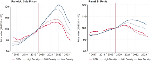
Similarly, Alipour and Krause (2025) find that while WFH contributed to some flattening of urban housing price gradients, the magnitude of these effects in Germany was considerably smaller than in the United States. The authors emphasize that the observed adjustments primarily reflect modest intra-urban reallocations of housing demand rather than fundamental changes in regional housing market dynamics. Alipour and Krause (2025) further provide additional support for the view that the omission of the COVID period is unlikely to affect the main conclusions of the present study. Figure 4, which is taken from Alipour and Krause (2025) documents a flattening of urban housing price and rent gradients in Germany between 2019 and 2023 but the magnitude of these adjustments is modest compared to the United States.

More importantly, the observed changes are concentrated within metropolitan areas, reflecting relative adjustments between central and peripheral locations rather than a fundamental restructuring of regional housing markets. In other words, the pandemic appears to have generated limited intra-urban reallocation of housing demand without substantially altering the broader spatial mechanisms governing land markets. This distinction is particularly relevant because our analysis focuses on county-level agglomeration effects and interregional spillovers. Therefore, although extending the sample to include the COVID-19 period would be essential, the available evidence suggests that the pandemic primarily affected relative housing demand within urban areas while leaving the broader regional structure of German land markets largely intact. We, therefore have little reason to expect that the estimated agglomeration and spillover effects identified through our spatial econometric framework would be materially altered by the inclusion of the COVID-19 period.

Taken together, these studies suggest that the German housing market remained relatively resilient to COVID-induced spatial restructuring. Consequently, we do not expect the pandemic to substantially alter the central conclusions of our paper regarding the role of agglomeration economies and spatial spillovers in land price determination.

Therefore, while extending the analysis to cover the COVID period would be a valuable direction for future research, it would address a distinct research question and require a different empirical framework. Given the objectives of the present study, the use of spatial econometric methods rather than a causal difference-in-differences design and the available evidence indicating limited COVID-induced spatial restructuring in Germany, we believe that such an extension would not materially alter the paper's main conclusions regarding the spatial determinants and spillover effects of land prices.

These findings have several implications. First, they reinforce the idea that land markets are central to understanding regional housing cycles and price divergence. Second, they highlight the importance of spatial structure, both in terms of economic geography and policy interdependence, when analyzing housing affordability and land use regulation. Finally, they suggest that spatial spillovers in land values should be explicitly incorporated into housing policy and planning models, particularly in rapidly growing urban regions.

The supplementary material for this article can be found online