Spatial dependence across US counties: an integrated gravitational, Moran and entropy-based approach

This study presents an empirical spatial analysis of the US market, focusing on mobile production factors, capital, and labor. The United States operates within a free-market capitalist system (Graafland and Verbruggen, 2022), which combined with its scale as the world's largest national market, positions it as a major contributor to the global GDP, making its evolution and global integration particularly relevant. This paper contributes to the literature by combining gravitational theory (focused on isolated bilateral flows), Moran-based spatial analysis, and entropy to interpret concentration and dispersion dynamics in the US economy, enabling a joint analysis of regional attraction and dependence. A distinctive feature of this work is the combination of an econophysical interpretation of gravitational forces with spatial econometrics techniques (Capoani et al., 2025). To ensure the robustness of clustering patterns, the model incorporates spatial weight matrices and applies permutation-based inference procedures for validation.

Across the history of economic thought and the social sciences, many concepts originally formulated within physical sciences – such as gravity and entropy – have been reinterpreted and adapted as analytical tools to provide a more scientific description of the social order.

First attempts in this direction can be found in Auguste Comte's idea of “physique sociale” and in Adolphe Quetelet's statistical approach in “Sur l'homme et le développement de ses facultés”. Building on this tradition, the formal introduction of gravitational reasoning into the analysis of socio-economic systems is commonly associated with the work of Stewart (1948), who first applied gravity-type models to social interactions, and was subsequently extended within regional science by Isard (1954), who provided a systematic framework for spatial economic analysis. Another notable example is offered by Wendt (2015), who suggests integrating elements of quantum mechanics into the ontology of social sciences.

This research aims to further develop the application of gravitational field theory (Capoani, 2023a) within international economics from an econophysical perspective, offering a framework to represent economic relationships while accounting for geographic distances. In this context, trade liberalization helps explain how the movement of goods and services and the reduction of trade barriers have shaped the US market, supporting regional exporters (Cooper, 2014).

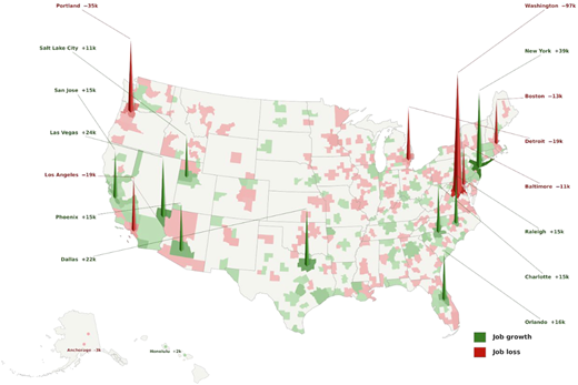
The study extends previous works by examining international market structures, regional dynamics, and clustering through the Moran Index – a widely used measure of spatial autocorrelation, applied here to analyze geographical patterns within the United States. It is used in this study to assess whether the observed spatial distribution of economic variables departs from randomness and exhibits systematic spatial dependence. Entropy-based measures (e.g. Shannon, 1948; Theil, 1967) provide valuable insights into dispersion and regional growth decomposition. This is particularly relevant in a country where economic activity is unevenly distributed and increasingly concentrated in major metropolitan areas and key regions, as also reflected in employment growth patterns in absolute value (Figure 1).

Over time, high-tech companies have concentrated in strategic regions, reducing economic distance through lower transportation and communication costs, a phenomenon described as the “death of distance” (Cairncross, 2002; Tranos and Nijkamp, 2013) consistent with the gravitational model. However, some authors find these assertions “premature” (Rietveld and Vickerman, 2004) and consider physical distance relevant (Brun et al., 2005).

Among these conceptual borrowings, gravity and entropy emerge as central analytical tools. While social physics applies physical principles to broad social phenomena, econophysics employs them in economic systems, emphasizing market dynamics, spatial interactions, and quantitative modeling.

Although they originate in different theoretical contexts (Newton's classical mechanism and thermodynamics), both have been adapted to analyze patterns of interaction, distribution, and organization in economics, contributing to the birth of econophysics.

Taken separately, they may appear incompatible: gravity can be interpreted as a force shaping interactions between units, while entropy relates to dispersion and the distribution of states within a system. Nevertheless, they can be treated as complementary principles of economic systems, capturing respectively the mechanism of concentration and dispersion.

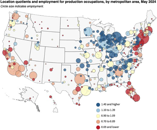
To operationalize this framework, the study employs a vector-based approach for analyzing regions and clusters, alongside a detailed examination of US counties. This approach – derived from the superposition principle – enables the quantification of gravitational fields and the analysis of interactions both between and within counties, going beyond the bilateral model. In this perspective, gravity can be interpreted as a bottom-up mechanism driven by interactions between individual units, while entropy reflects a top-down constraint shaping the system's overall configuration. The model also explains patterns in American urban centers. These areas host highly innovative and value-adding sectors and contribute disproportionately to national GDP and economic growth, particularly across coastal areas and parts of the Midwest and Great Plains (Atkinson et al., 2019). This supports a broader winner-take-all dynamic, whereby more developed regions attract further talent, investment, and innovation. The gravitational framework provides an interpretation of spatial economic attractiveness among states and regions by describing how population density and distance influence economic attractiveness. This mechanism is evident in the role of large metropolitan areas in driving economic activity, as reflected in employment and location quotients across US metropolitan regions (Figure 2); the largest US metropolitan areas account for approximately one-quarter of national GDP, reflecting the strong concentration of economic activity in urban regions.

(Source: US Bureau of Economic Analysis, GDP by Metropolitan Area).

While the county level remains the core unit of analysis in the empirical sections, metropolitan areas are used here for descriptive illustration of broader concentration patterns.

Table 1 provides a comparative framework of gravitational, Moran-based, and entropy-based approaches, highlighting their distinct yet related analytical roles, outputs, and economic interpretations in the analysis of concentration and dispersion dynamics.

This paper is structured into four sections. It begins with the theoretical framework, focusing on how gravitational models can be integrated with spatial analysis, followed by a discussion of the data and methodology, including the construction of spatial weight matrices and the application of Moran's I and entropy models. After discussing the empirical findings, the paper concludes with a summary of the results and their implications for future research.

Overall, this study proposes a methodological tool for analyzing regions, clusters, and, specifically, US counties by using vectors to map economic interactions and dynamics.

The United States represents a suitable case study due to its large and heterogeneous economic space, with significant regional disparities and high factor mobility. Moreover, the availability of detailed county-level data enables a fine-grained spatial analysis, enabling the identification of localized patterns that would be less observable in smaller-scale regional contexts.

In this chapter, we present an integrated empirical analysis of spatial economic dynamics in the United States by combining complementary methodological approaches: we employ Moran's I to identify and localize spatial clustering patterns, entropy measures to assess the overall degree of concentration or dispersion of economic activity, and a gravity-based interpretation to capture the forces of economic attraction across regions. County-level socioeconomic data were obtained from the Bureau of Economic Analysis (BEA), while spatial boundary files were obtained from the US Census Bureau. Complete references and URLs for these datasets are provided in the  Appendix. This multi-dimensional interpretation of regional economic structures identifies where economic activity is concentrated, how it is distributed at the aggregate level, and which mechanisms shape its spatial configuration, linking empirical evidence to an economic interpretation of spatial interactions. GDP and population are employed as proxy measures of economic “mass” within the gravitational framework, as they directly reflect the scale and intensity of economic activity. While GDP captures the overall economic output, population accounts for the distribution of human capital and potential labor supply, both of which contribute to regional attractiveness. To move beyond purely size-based measures, we introduce the Financial Performance Index (FPI), which provides a synthetic indicator of economic performance and local efficiency, allowing us to capture regional qualitative differences that are not fully reflected by aggregate variables. Finally, net migration is included as a behavioral variable, representing the actual response of individuals to spatial economic conditions. In this sense, it serves as an observable outcome of underlying economic forces, linking structural attractiveness to real population movements. These integrated variables enable a multidimensional representation of economic space, balancing structural, performance-based, and dynamic perspectives (all analyses were conducted using R and Python for spatial computation, data processing, and visualization).

In this section, we introduce a gravity-based approach aimed at analyzing the structure of economic attraction across space. This framework is grounded in the tradition of Stewart and Isard's gravitational models in economics – later reconstructed by Capoani (2023b, 2024) – in which economic interactions are modeled in analogy with the laws of physical gravitation. Indeed, the economic literature has progressively developed the concept of economic potential, according to which the attractiveness of a region depends on the economic mass of other regions and the distance separating them. Within this framework, the formulation of income potential can be expressed as:

where $Yj$ represents the income of region $j$⁠, and $dij$ denotes the economic distance between regions. This formulation allows economic interactions to be interpreted as the cumulative outcome of multiple spatial influences. In parallel, the analogy with physics suggests representing economic interactions in terms of gravitational forces, which can be formally expressed as:

where $Mi$ and $Mj$ represent the economic masses of regions, and $Dij$ denotes the distance between them. However, this formulation remains inherently bilateral and does not fully capture the systemic nature of economic interactions. To overcome this limitation, we adopt a scalar representation based on the principle of superposition, which allows the aggregation of the influence exerted by all regions on a given territorial unit. Within this framework, we define the Integrated Gravitational Potential Gradient (IPG) as:

where $Mj$ denotes the economic mass of region $j$⁠, $dij$ is the distance between regions, and $α$ represents the distance decay parameter (set equal to 1 in the baseline specification). This formulation enables a shift from a bilateral perspective to a multilateral and systemic representation, in which the attractiveness of each region is determined by the cumulative effect of spatial interactions. As a result, the proposed approach allows for the identification of the main poles of economic attraction and supports the analysis of the spatial structure of the economic system as a whole, overcoming the limitations of approaches based exclusively on local relationships or pairwise regional interactions.

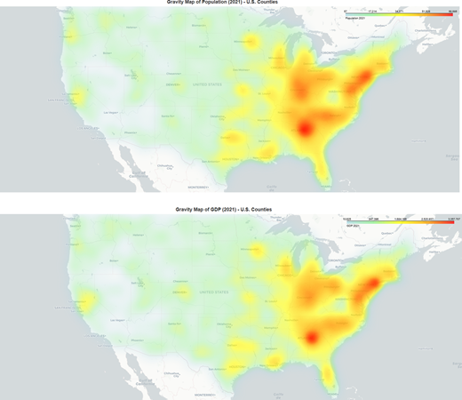
Consistent with the theoretical framework of the gravitational model introduced above, the IPG analysis is applied to variables expressed in absolute terms, namely population and GDP. As discussed, the use of “mass” variables allows for a more accurate representation of the attractiveness of territories, avoiding the distortions that would arise from the use of relative variables, which could assign similar levels of “attractiveness” to regions that differ substantially in size. Both resulting maps (Figure 3) reveal a clear concentration of the gravitational field in the eastern territories, with a high-attractiveness area extending along the East Coast and an intense core in the North-East, corresponding to the New York-Philadelphia-Boston corridor. This is accompanied by an additional significant pole in the South-East, centered on the Atlanta area, as well as an intermediate band of attractiveness involving parts of the Midwest and the Great Lakes region, with notable contributions from cities such as Chicago and Detroit.

The emerging spatial structure is not characterized by isolated poles, but by a continuous gravitational field, in which the superposition of effects (principle of superposition) generates an extended area of high attractiveness. This is evident in the maps, where high-intensity areas appear interconnected, outlining a systemic configuration of economic and demographic activity. In contrast, the West Coast exhibits a more fragmented and discontinuous distribution. Although relevant poles are observable – especially in California and the Pacific Northwest – these appear more isolated and less integrated within a diffuse gravitational field, highlighting a structural difference between the two coasts: an extended and interconnected system on the East Coast, versus a more localized and discontinuous configuration on the West Coast.

From a methodological perspective, winsorization at the 75th percentile limits the influence of extreme observations, preventing few high values from dominating the spatial representation. This enhances the readability of the structural component of the phenomenon, emphasizing systemic patterns rather than merely local anomalies. The comparison between the two variables reveals consistent results: both population and GDP delineate a gravitational field strongly concentrated in the eastern regions. This supports the interpretation that economic and demographic density plays a central role in the formation of attraction poles, confirming the validity of the gravitational model for analyzing spatial dynamics.

The gravitational analysis thus provides a continuous and systemic representation of economic attraction forces, allowing the identification of the main poles of concentration and areas of stronger spatial interconnection. However, while this approach captures the intensity and distribution of the “economic field”, it does not allow us to determine whether such concentrations translate into statistically significant clustering patterns at the local level. For this reason, in the next step, we complement the analysis with spatial autocorrelation tools, which formally identify the presence of clusters and local structures within the economic system.

While the gravitational model captures the overall structure of economic attraction and the intensity of spatial interactions, it provides a continuous depiction of the economic field. To shift from a systemic, “smooth” representation to a statistically rigorous identification of local patterns, a measure of spatial autocorrelation is required. In this regard, Moran's I serves as a natural extension of the analysis, allowing the formal identification and classification of clusters and outliers in geographic space.

In this section, we apply the Moran Index and gravity maps derived via vector superposition to examine spatial economic patterns across US counties. The global Moran Index provides a measure of overall spatial clustering, whereas the local Moran analysis identifies geographically specific clusters, allowing for a detailed territorial interpretation. With over 3,000 counties included per variable, the dataset offers a high level of regional granularity, enhancing the detection of local clusters relevant for policy analysis. A crucial element in the computation of Moran's I is the definition of the spatial weights matrix, which establishes the pattern of spatial interactions among counties. For this study, we adopt a contiguity-based approach, specifically a queen criterion, whereby two counties are considered neighbors if they share either a boundary or a vertex. This choice is consistent with the administrative and geographical configuration of US counties and enables us to capture both direct and indirect spatial interactions. Although alternative specifications – such as distance-based weights or k-nearest neighbors – are possible, contiguity-based weights are particularly suitable for capturing localized spillover effects in territorial economic systems.

The data used in this study are obtained from the US Bureau of Economic Analysis and the US Bureau of Labor Statistics. Both global and local Moran analyses rely on a spatial weights matrix, which specifies the interactions among spatial units. We adopt a “queen” contiguity criterion, where counties are considered neighbors if they share a boundary or vertex. This choice aligns with the administrative organization of the dataset and accounts for the influence of geographical proximity in economic interactions. Although alternative specifications – such as distance-based weights or k-nearest neighbors – could be applied, contiguity-based weights are more appropriate in this context. While different weighting schemes may influence the intensity of spatial autocorrelation, clustering patterns remain qualitatively stable. Geographic data are sourced from US Census Bureau shapefiles, limited to the 48 contiguous states and Washington D.C.

Statistical significance is assessed using permutation-based pseudo p-values, which approximate the probability of observing statistics as extreme as the observed ones. To reduce false positives, we adopt a conservative threshold (α = 0.001), then we validate the results using the False Discovery Rate (FDR) approach. Specifically, pseudo p-values are ranked in ascending order and compared to the FDR threshold computed as:

where I is the rank of the ordered pseudo p-values and n is the total number of observations. An observation is statistically significant if its pseudo p-value is lower than the corresponding FDR value. The two approaches yield consistent results, confirming the robustness of the identified clusters. Counties are classified into four categories: “high-high” and “low-low” clusters, and “high-low” and “low-high” spatial outliers, allowing the identification of both concentration patterns and spatial anomalies across the territory.

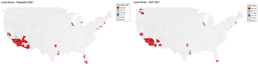
The analysis considers population and GDP (in current dollars) as proxies for economic mass, alongside production factors, such as labor and capital, with the aim of identifying the main centers of economic attractiveness. The global Moran Index computed for the 2021 US population is equal to 0.3764, indicating statistically significant spatial clustering. However, the global measure shows limited robustness; removing the top 1% of observations increases the index by 7.49%. By contrast, the local Moran analysis offers a more accurate representation of spatial patterns. Results highlight clusters concentrated in major urban and metropolitan areas, corresponding to the main US economic centers. Figure 4 reports the local Moran cluster map for population and GDP in 2021. Comparing the fixed pseudo p-value threshold (0.1%) with the FDR approach shows consistent findings: 87 observations are identified under the fixed threshold, while 71 and 91 observations are identified using FDR with α equal to 1 and 5%, respectively. This suggests that the 0.1% threshold corresponds to an effective significance level between 1 and 5%, in line with standard practices in economic and social science research. Accordingly, county significance in the local Moran cluster map (Figure 4) is set at 0.1%, ensuring a conservative and robust identification of spatial clusters.

Besides population, the second variable (Figure 4) is the absolute GDP value in thousands of current 2021 dollars by county.

The two visualizations appear very similar, with the coastal regions dominating the maps. As anticipated, the significant clusters identified are almost exclusively “high-high” clusters, located near major US cities: along the East Coast (New York, Philadelphia, Boston, and Washington D.C.) to the West Coast (Los Angeles, San Diego, and Seattle only for nominal GDP), the Lakes area (Chicago and Detroit only for population), Florida (Miami and Orlando-Tampa area only for population) to Texas (Houston and Dallas), and Atlanta (only for nominal GDP), with the largest clusters concentrated in California. While one might attribute it to the larger size of counties there compared to the East Coast, this explanation does not account for the San Francisco Bay Area, which constitutes an extensive cluster composed of many relatively small counties. Additionally, the maps demonstrate that county populations–ranging from a few hundred to several million inhabitants–heavily influence clustering patterns for GDP and its variability; hence, population may act as a confounding factor in these analyses if not properly considered. Nevertheless, population mapping is relevant for our purposes and for understanding economic and commercial gravity centers' location over the US territory.

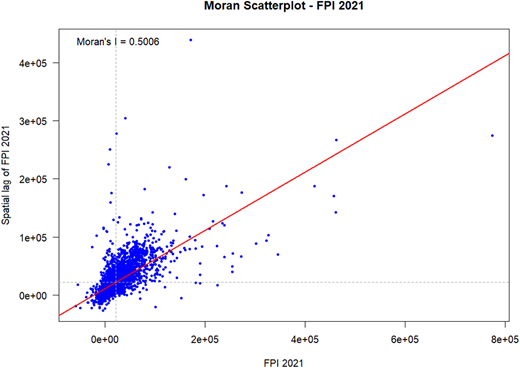
To deepen the analysis of spatial economic dynamics, we extend the investigation by considering two additional variables: the Financial Performance Index (FPI) and net migration. The FPI reflects the economic performance and local economic strength of each county, serving as an indicator of its relative attractiveness. Net migration, instead, measures the actual inflow or outflow of the population, representing how individuals respond behaviorally to spatial economic conditions. The FPI offers a composite measure of economic performance and local appeal beyond sheer economic size. The global Moran's I for 2021 FPI is equal to 0.5006, indicating a statistically significant degree of spatial autocorrelation. This result suggests that economically performing counties are geographically clustered and tend to be surrounded by areas with similar levels of performance.

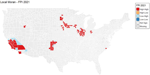
The Moran scatterplot (Figure 5) shows that counties with high FPI value are positively associated with high values of the corresponding spatial lag. The slope of the fitted line reinforces the presence of strong spatial dependence. Moreover, the local Moran cluster map for FPI (Figure 6) identifies significant “high-high” clusters, notably in California as well as in multiple metropolitan areas across the Midwest and selected inland regions.

These clusters identify key economic centers characterized by their size and high levels of economic performance. Compared to GDP, FPI highlights a more articulated spatial structure, capturing areas of economic strength that extend beyond the traditional coastal hubs. To complement this analysis, net migration is examined as a dynamic indicator of regional attractiveness. While GDP and FPI capture the economic “mass” and performance of a region, net migration reflects the actual movement of individuals responding to spatial economic incentives.

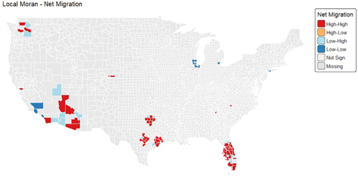
The local Moran cluster map for net migration (Figure 7) highlights significant “high-high” clusters in regions such as Florida, Texas, and parts of the Southwest, indicating strong population inflows. Conversely, “low-low” clusters emerge in portions of the Midwest and northern regions, reflecting persistent outflows. These patterns suggest that migration can be interpreted as a behavioral response to underlying economic forces: economically dynamic and attractive regions exert centripetal effects, attracting inflows, whereas less dynamic areas display centrifugal tendencies associated with population decline. From this perspective, net migration provides empirical validation for the gravitational framework, representing the observable manifestation of spatial economic forces, translating differences in economic performance into actual movements of population across regions.

Moran's analysis provides a detailed and statistically grounded representation of the spatial organization of economic activity, emphasizing the presence of local clusters and their geographic distribution. Nonetheless, while this approach is highly effective in detecting spatial dependencies and local patterns, it does not yield a synthetic measure of the overall distribution of economic activity within the system. Hence, Moran's I provides insight into the location of clusters, but does not quantify the degree to which economic activity is concentrated or dispersed at the national level.

To complement both the local perspective provided by Moran's I and the interaction-based framework of the gravitational model, we employ an entropy-based framework to quantify the degree of dispersion of economic activity across the United States. Whereas the gravitational model focuses on attraction forces between areas and Moran's I identifies local spatial autocorrelation patterns, entropy provides a synthetic measure of the overall distribution of economic mass among regions. We adopt the normalized Shannon entropy, computed on the distribution of economic variables across states. For a given variable, the entropy index is defined as:

where $pi$ represents the share of the $i$-th state relative to the national total of the variable considered, and $N$ denotes the total number of states. The normalization by $ln(N)$ ensures that the index ranges between 0 and 1, allowing for direct comparability across variables defined on different spatial partitions.

While entropy provides a measure of dispersion, in the empirical analysis we adopt an interpretation in terms of internal concentration. In this perspective, lower entropy values correspond to a higher concentration of economic or demographic activity within a limited number of counties, whereas higher entropy values indicate a more homogeneous spatial distribution across the territory. This interpretation allows us to directly assess the degree of internal imbalance within each state. Within this framework, entropy complements the gravitational and Moran-based approaches. The gravitational model captures the centripetal forces driving economic concentration, while Moran's I identifies local clusters and spatial dependencies. Entropy, by contrast, provides a global and synthetic measure of how economic and demographic mass are distributed within the system. This approach enables a comparison between the spatial distribution of population and economic activity across states, highlighting differences in the degree of internal concentration. The integration of gravitational interactions, local spatial autocorrelation, and entropy-based measures thus offers a comprehensive interpretation of spatial economic dynamics, combining local interactions, global distribution patterns, and the balance between forces of concentration and dispersion. Within this framework, entropy complements both the gravitational approach and Moran's I. The gravitational model captures the centripetal forces driving economic concentration, while Moran's I identifies local clusters and spatial dependencies. Entropy, in contrast, provides a global measure of dispersion within the system, capturing centrifugal dynamics at the national scale. The entropy index is computed for both population and GDP, enabling a comparison between the distribution of demographic and economic mass across states. This comparison highlights spatial inequalities, indicating whether economic activity is more concentrated than population, or vice versa. The integration of these approaches enables a more comprehensive interpretation of spatial economic dynamics, combining local interactions, global distribution patterns, and the balance between forces of concentration and dispersion.

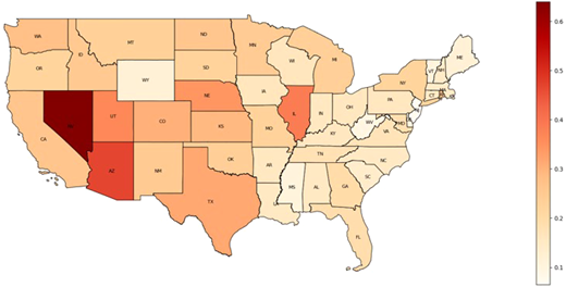
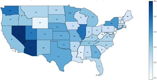
Based on the framework described above, the entropy measure allows for a geographic interpretation of the distribution of economic and demographic mass. The maps presented below (Figures 8 and 9) display the values of the polarization index for each state, based on normalized entropy. This measure captures the degree of concentration of economic and demographic activities within each state, thereby allowing the identification of areas characterized by higher internal imbalances. With regard to population, a relatively low level of polarization emerges across most states, indicating a fairly balanced spatial distribution of residents among counties. Only a limited number of states exhibit moderately higher values, suggesting some degree of concentration in major urban areas. Overall, the evidence points to a relatively homogeneous demographic structure, consistent with a high level of entropy and the absence of strong internal polarization.

The analysis of GDP, by contrast, reveals a markedly different spatial pattern. Several states exhibit significantly higher levels of polarization, indicating that economic activity is strongly concentrated within a limited number of counties. In particular, states such as Nevada, Arizona, Illinois, and New York display elevated values, reflecting the presence of dominant economic hubs, often large metropolitan areas, that generate a substantial share of total output. This pattern suggests that, within these states, economic production is not evenly distributed across the territory but is instead driven by a small number of highly productive areas. Conversely, many other states show relatively low levels of polarization, indicating a more balanced internal structure in which economic activity is more evenly spread across counties, without a single dominant center. Overall, this evidence highlights a heterogeneous economic structure across the United States, where highly concentrated systems coexist with more territorially balanced ones. This distinction is particularly relevant from a spatial perspective, as it reflects differences in the organization of production, the role of urban agglomerations, and the extent to which economic activity is localized within specific regional hubs.

The comparison between the two maps highlights a clear structural divergence between demographic and economic patterns. While population is relatively evenly distributed within states, GDP exhibits a higher degree of internal concentration, indicating that economic value creation is more spatially clustered than population, reflecting localized production centers and agglomeration effects. These findings are consistent with the Moran analysis, which identified local clusters of high economic activity, and with the gravitational framework, which emphasizes attraction forces between economically relevant regions. In this context, the polarization index complements these approaches by providing a synthetic measure of internal concentration, enriching the interpretation of spatial economic dynamics. Overall, the US system is characterized by a relatively balanced demographic distribution, alongside a more polarized economic structure. The integration of entropy, spatial autocorrelation, and gravitational models thus provides a comprehensive framework for understanding territorial dynamics, highlighting the interaction between centripetal (concentration) and centrifugal forces (dispersion) in shaping economic space.

This paper develops an integrated framework for the analysis of spatial economic dynamics, combining gravitational modeling, spatial autocorrelation, and entropy-based approaches, in line with the main theoretical strands discussed in the literature.

In particular, this contribution builds upon the established tradition of gravity models in spatial economics, as well as on the literature on spatial dependence and entropy-based measures. While these approaches have typically been applied separately, this study proposes a unified perspective in which they are jointly employed to interpret spatial economic structures. Each method captures a specific component of the territorial system, making it clear that their combined use is not redundant, but essential for a comprehensive representation. More specifically, the gravitational model identifies economic attraction forces and the continuous structure of the spatial field, highlighting macro-poles and areas of strong interconnection, especially along the East Coast. Moran's analysis, in contrast, provides a discrete and statistically grounded interpretation, identifying significant local clusters and confirming the presence of spatial concentrations of economic activity. The entropy-based approach complements this analysis by offering a synthetic measure of the internal distribution of economic and demographic activity, capturing differences in the degree of concentration across states and revealing a structural divergence between demographic and economic patterns.

These findings are consistent with the theoretical expectation that economic activity is not randomly distributed in space, but tends to organize itself through cumulative processes of interaction and spatial dependence, as highlighted in the existing literature.

While the proposed conceptual framework provides significant insights into spatial economic dynamics, some limitations should be acknowledged. The cross-sectional nature of the analysis does not fully capture the temporal evolution of spatial patterns. Furthermore, results may vary depending on the specification of the spatial weighting matrix, and the set of variables considered, while relevant, does not encompass all dimensions of regional development. These aspects do not weaken the approach, but rather highlight the value of combining multiple analytical perspectives.

The comparison of these three approaches therefore underscores their profound complementarity. The gravitational model captures interaction forces between territories, Moran's I identifies local clustering patterns, and entropy captures the overall distribution of economic and demographic mass, allowing for an assessment of the degree of internal concentration within each state. When considered in isolation, each of these tools provides only a partial view of the phenomenon; when integrated, they enable a multi-level interpretation of spatial dynamics, in which interactions, local dependencies, and overall distribution are jointly analyzed. From a methodological perspective, this study contributes to the literature by proposing an integrated framework that combines gravitational models, spatial autocorrelation, and entropy-based measures within a single analytical structure. This integration represents an advancement over traditional approaches, which tend to consider these tools separately, and allows for overcoming the limitations of individual methodologies. In particular, it helps avoid partial or distorted interpretations, providing a more robust and coherent view of territorial dynamics.

From an empirical standpoint, the results show that the US economic system is characterized by a strong concentration of productive activity in a limited number of poles, alongside a relatively more dispersed population distribution. This evidence suggests the presence of economic agglomeration mechanisms that are not proportionally reflected in demographic patterns, contributing to spatial inequalities and territorial divergence.

The integration of the gravitational approach, Moran's I, and entropy therefore makes it possible to interpret spatial economic dynamics as the result of the interaction between centripetal and centrifugal forces, providing a more comprehensive and coherent analytical framework. This approach proves particularly relevant not only for academic analysis but also for policy implications, as it allows for a more precise identification of areas of concentration, zones of fragility, and potential drivers of territorial development.

Overall, the paper contributes to the literature by integrating gravitational models, spatial autocorrelation, and entropy-based approaches into a coherent analytical framework, thereby extending existing perspectives on the study of spatial economic dynamics.

The authors were solely responsible for the conception and design of the study, acquisition, and analysis of data, and drafting of the manuscript.

This article does not contain any studies with human participants performed by the authors.

Not applicable as this study did not involve human participants.

Not applicable as this study did not involve human participants.

We thank the European Youth Think Tank cultural association for providing a stimulating context for the development of our collaboration in this article.

Data sources:

1. County-level data about (Population, GDP in current thousands of USD, and Per capita dividends, interest, and rent) Bureau of Economic Analysis (BEA); U.S. Department of Commerce. Available at: Link to the website.

2. County-level shapefiles (U.S. cartographic boundaries):

   United States Census Bureau. Cartographic Boundary Files. Available at: Link to the website.