


In this paper, the heterogeneity of the linkages among financial development, productivity and growth across income groups is emphasized.
An empirical analysis is conducted with an illustrative sample of 130 economies over the period 1991–2019 and classified into four subsamples: Organisation for Economic Co-operation and Development (OECD), developing, least developed and net food importing developing countries. Forecast error variance decompositions and panel vector auto-regressive estimations are computed, with insightful findings.
Higher levels of output stimulate the economic development in the agricultural sector, mainly via the productivity channel and, in the most developed economies, also through access to credit. Differently, in developing and least developed economies, the role of access to credit is marginal. The findings have practical implications for stakeholders involved in the planning of long-run investments. In less developed economies, priorities should be given to investments in technology and innovation, whereas financial markets are more suited to boost the development of the agricultural sector of developed economies.
The authors conclude on the credit–output–productivity nexus and contribute to the literature in (at least) three ways. First, they assess how credit access, agricultural output and agricultural productivity are jointly determined. Second, they use a novel approach, which departs from most of the case studies based on single-country data. Third, they conclude on potential causality links to conclude on policy implications.
1. Introduction
The agricultural sector and its economic development are tightly linked to innovations, investments and the use of capital-intensive inputs (Farrokhi and Pellegrina, 2023). More than other sectors, the agricultural sector is vulnerable to different types of risks, and their management has been, for decades, a priority in the policy agenda, with interventions devoted to subsidizing participation in insurance markets (Goodwin, 2001; Santeramo, 2019; Chopra et al., 2022; Santeramo et al., 2022), the adoption of instruments to stabilize revenues and incomes (Klimkowski, 2016; Cordier and Santeramo, 2020), and the access to credit (Salami et al., 2013; Martin and Clapp, 2015). This last aspect has received, compared to other topics, relatively less attention, whereas it may represent a strong driver for development, allowing farmers to purchase inputs, plan investments and face monetary shocks. As argued in several studies (e.g. Azariadis and Drazen, 1990), “economies with credit rationing tend to experience slower growth [ …] than will an otherwise identical economy with perfect credit markets”.
The need for credit access is particularly important for farmers who face a time lag between expenditure on crop cultivation (i.e. perennial crops) and the realization of revenues from the sale of their products. Credit is expected to become even more important due to the emergence of new environmentally related risks (e.g. climate risks), which will affect land values, output and productivity (Ay and Latruffe, 2017). According to World Bank (WB) data, despite its importance, the total credit to agriculture disbursed by commercial banks has been below 3% in 2017, which is lower than the contribution of the agricultural sector to the global Gross Domestic Product (GDP). More worrisome, the global share of agriculture in total credit is steadily falling, from 2.50% in 2012 to 2.14% in 2021 (Food and Agriculture Organization (FAO), 2022). The agricultural sector receives less money than the value it generates.
Besley (1994) provided several theoretical arguments to explain market failures (e.g. imperfect information and learning curve) and justify policy interventions to improve credit access in rural economies. He argues that “it is impossible to be categorical that an intervention in the credit market is justified.”
The credit access and economic growth nexus has been widely investigated (Karlan and Morduch, 2010); notwithstanding, there is no consensus on the causal links: economic growth spurs credit access. Moreover, credit access can spur growth (Magazzino et al., 2021a). Levine (2005) reviewed the empirical associations across fundamentals and showed that the connection between credit access and economic growth cannot be justified merely through a reverse causation relationship. Indeed, cross-country regression analyses support the tight link between credit access and economic growth (Rajan and Zingales, 1998; Beck et al., 2000), both for developed and developing economies (Levine et al., 2000; Winter-Nelson and Temu, 2005). Other cross-countries studies support evidence of reciprocal effects (Zang and Kim, 2007; Baliamoune-Lutz, 2013). Thus, while the empirical literature draws conclusions on the financial development–economic growth nexus, the evidence on the direction of causality is lacking.
A further strand of the literature has investigated how credit access, agricultural output and agricultural productivity are linked together (Feder et al., 1990; Rozelle et al., 1999; Foltz, 2004; O'Toole et al., 2014; Howard and Livermore, 2021). Most studies are country-specific analyses that focus on dyad relationships. The literature has two topics missing. The first is the extent to which credit access, agricultural output and agricultural productivity are jointly determined. In addition, there is a lack of consensus on the direction of causalities operating among financial, productivity and economic indicators. Against this background, we pose two research questions: (1) how do access to credit, output and productivity covary? (2) How do these dynamics differ across countries with heterogenous levels of economic development?
The main methodological challenges that past investigations have attempted to address so far are highlighted from both historical and statistical perspectives. Our attempt is to reconcile the conflicting findings. This study finds its second innovative contribution by taking a representative sample of 130 economies as a global illustrative case and revisiting the dynamic relationship among credit access, productivity and output in the agricultural sector. The paper displays a last competitive edge as it employs a recent panel data methodology (i.e., Panel Vector Auto-Regressions, PVAR), thought to remedy past methodological issues and offer more robust estimates for policy purposes (Magazzino, 2014).
Data span the largest available period: 1991–2019. To the best of our knowledge, this paper is among the very few (if not the only one) in assessing the above nexus for an illustrative panel of 130 countries using a PVAR methodology. We account for income level heterogeneity among countries. Thus, we also stratified the empirical analysis with four distinct subsamples: least developed, net food importing developing (NFID), developing and Organisation for Economic Co-operation and Development (OECD) member countries. This study contrasts with previous ones as it employs a stepwise econometric causality testing framework constituted of paired sample statistics, PVAR estimates from Cagala and Glogowsky (2014) – which are more reliable than standard methods when dealing with statistical identification problems – and forecast error variance decompositions (FEVDs).
We conclude on the credit–output–productivity nexus and contribute to the literature in (at least) three ways. First, we assess how credit access, agricultural output and agricultural productivity are jointly determined. Second, we use a novel approach, which departs from most of the case studies based on single-country data. Third, we conclude on potential causality links to conclude on policy implications.
Associated insights are expected to help further understand the channels through which financial, productivity and sectoral performance indicators connect and interact in the agricultural sector. Notably, our estimates provide strong empirical support to Verdoorn’s law (Verdoorn, 1949) [1], since the output variable turns unanimously statistically significant in the productivity equation, regardless of the income group considered.
2. Data collection and methodology
To implement our empirical methodology, data series related to credit, productivity and sectoral output variables are collected [2].
The applied analysis uses annual data from 1991 to 2019 and computes series for a global illustrative sample of 130 economies. LAGTFP represents the agricultural total factor productivity (TFP) index using primarily USDA data. LRCA refers to the credit to agriculture, in US $, at constant prices. LGAO corresponds to the gross agricultural output for each country, where annual fluctuations have been smoothed by the Hodrick–Prescott filter. The data are derived from the USDA and the FAOSTAT databases [3]. The data starting period was dictated by credit to agriculture data availability. Moreover, we avoided the more recent years, since the current economic–financial crisis has substantially affected the estimated relationships. We derived the log-transformation of all variables. Table A1 in Appendix summarizes the variables considered in the empirical analysis.
Descriptive statistics
| Variable | Mean | Median | Std. Dev | Skewness | Kurtosis | Range | IQR | CV |
|---|---|---|---|---|---|---|---|---|
| LAGTFP | 4.5270 | 4.5566 | 0.2192 | −0.4101 | 5.1340 | 1.9267 | 0.2210 | 0.0484 |
| LRCA | 9.0839 | 8.9248 | 2.7889 | 0.1692 | 2.5458 | 15.6677 | 4.2568 | 0.3070 |
| LGAO | 15.2733 | 15.2351 | 1.8958 | −0.0071 | 2.9342 | 10.4577 | 2.3434 | 0.1241 |
Note(s): Std. Dev.: Standard Deviation; IQR: Interquartile Range; CV: Coefficient of Variation
Source(s): Authors’ calculations
A graphical analysis of the three variables of interest (Figure 1) allows us to conclude on overall correlations. The scatterplot matrices show that the gross agricultural output and the agricultural TFP index are barely correlated. The credit to the agricultural sector is positively correlated with the gross output but not with the agricultural TFP index.
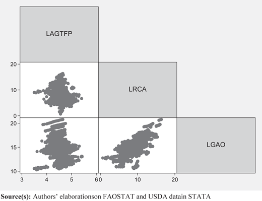
Agricultural TFP index, credit to agriculture, and gross agricultural output in 130 countries (1991–2019, log-scale)
Agricultural TFP index, credit to agriculture, and gross agricultural output in 130 countries (1991–2019, log-scale)
Table A1 in Appendix reports the summary statistics for the overall sample. The mean value of all variables is positive. Agricultural productivity and gross agricultural output have a negative value of skewness, indicating that the distribution is left-skewed. In addition, it is interesting to note how these three variables show similar values for mean and median in each subsample, indicating that a normal distribution emerges. Since, for each variable, the 10% trimmed mean values are near the mean, as well as the standard deviation to the pseudo standard deviation, the interquartile range (IQR) shows the absence of outliers in the observed sample. Moreover, correlation coefficients (r) are positive and significant at a 1% level in each subsample.
In addition, in Table A3 in the appendix, we provide some evidence of mean or median comparison tests. The results clearly underline how these values for the credit access variable statistically differ in all different subsamples. In fact, the null hypothesis is rejected everywhere. These findings provide further support that estimating the model in the different selected subsamples is reasonable and it can provide additional evidence.
Paired samples statistics
| Variable | Groups | Mean | N | Standard error | Standard deviation | t | Satterthwaite’s d.o.f | Wilcoxon test | Kruskal–wallis test | One-way ANOVA F test | Pearson χ2 test | Kolmogorov–Smirnov test |
|---|---|---|---|---|---|---|---|---|---|---|---|---|
| 1. LRCA | Non-OECD | 8.60 | 2,224 | 0.0545 | 2.5718 | −33.19 | 548.778 | −22.137 (0.0000) | 490.055 (0.0001) | 659.60 (0.0000) | 315.286 (0.000) | 0.6286 (0.000) |
| OECD | 12.36 | 330 | 0.0995 | 1.8084 | ||||||||
| 2. LRCA | Non-developing | 11.25 | 601 | 0.1349 | 3.3063 | 19.70 | 773.148 | 20.499 (0.0000) | 420.216 (0.0001) | 583.40 (0.0000) | 275.768 (0.000) | 0.5484 (0.000) |
| Developing | 8.42 | 1,953 | 0.0502 | 2.2181 | ||||||||
| 3. LRCA | Non-NFID | 9.36 | 1,939 | 0.0675 | 2.9711 | 11.51 | 1665.920 | 8.102 (0.0000) | 65.646 (0.0001) | 83.52 (0.0000) | 32.932 (0.000) | 0.3031 (0.000) |
| NFID | 8.20 | 615 | 0.0749 | 1.8586 | ||||||||
| 4. LRCA | Non-LD | 9.63 | 2,021 | 0.0618 | 2.7796 | 28.09 | 1465.070 | 20.341 (0.0000) | 413.751 (0.0001) | 433.00 (0.0000) | 414.267 (0.000) | 0.5027 (0.000) |
| LD | 7.02 | 533 | 0.0695 | 1.6050 |
Note(s): Unequal variances assumed, after some checks. After ANOVA, Sidak multiple-comparison test has been performed. P-Values in parentheses. Wilcoxon test: Two-sample rank-sum Mann–Whitney test. Kruskal–Wallis test: χ2 test with ties. Pearson χ2 test: Median test, continuity corrected. Kolmogorov–Smirnov test: Two-sample test for equality of distribution functions
Source(s): Authors’ calculations
The time-series econometric strategy uses a PVAR methodology from Cagala and Glogowsky (2014), thought to be more reliable than standard methods when notably dealing with statistical identification problems. This technique combines the traditional vector auto-regressions (VAR) approach, which treats all the variables in the system as endogenous, with the panel data approach, which allows for unobserved individual heterogeneity. Moreover, this procedure is insensitive to the order of the variables in the PVAR system. A first-order VAR model is specified as follows:
where ωit is a three-variable vector , fi is a 3*1 country-specific intercept term (fixed effect), dct corresponds to country-specific time dummies, Φ1 is a 3*3 coefficient matrix, and εit is a 3*1 residual term. We use to index countries and t to index time. The estimates describe the reaction of one variable to the innovations in another variable in the system, while holding all other shocks equal to zero. The identifying assumption is that the variables that come earlier in the ordering affect the following variables contemporaneously, as well as with a lag, while the variables that come later affect only the previous variables with a lag (Magazzino, 2016). In other words, the variables that appear earlier in the systems are more exogenous and the ones that appear later are more endogenous. In our specification, we assume that current shocks to the agricultural TFP influence the contemporaneous value of credit to agriculture, while the latter influences gross agricultural output only with a lag. Moreover, we assume that credit to agriculture responds to gross agricultural output contemporaneously, while the latter responds to agricultural TFP only with a lag. Our main objective is to compare the dynamics of credit access and its relationships with agricultural output and agricultural productivity.
To avoid the problem of correlation between fixed effects and regressors, we use forward mean-differencing, also referred to as the Helmert procedure (Holtz Eakin et al., 1988; Arellano and Bover, 1995), which removes only the forward mean. The coefficients are estimated by the System Generalized Method of Moments (GMM-Sys) (Blundell and Bond, 1997). Our model indeed allows for country-specific time dummies, dct, which are added to the model (1) to capture aggregate, country-specific macro shocks that may affect all countries in the same way. These dummies have been dropped by subtracting the means of each variable calculated for each country-year (Magazzino, 2017). In addition, standard errors of the impulse-response functions and confidence intervals have been calculated through Monte Carlo simulations [4] (Love and Zicchino, 2006).
We implemented the estimator suggested by Cagala and Glogowsky (2014), which runs a multivariate panel regression of each dependent variable on lags of itself and on lags of all the other dependent variables using the least squares dummy variable estimator (LSDV). Finally, we present variance decompositions, which show the percentage of the variation in one variable that is explained by the shock to another variable, accumulated over time. The variance decompositions show the magnitude of the total effect. We report the total effect accumulated over 10, 20 and 30 years, as longer time horizons produced equivalent results.
3. Empirical results
We estimate the coefficients of the system after the fixed effects and the country-time dummy variables have been removed. We show in Table A2 in the appendix the results of Fisher-type panel unit-root tests (Choi, 2001) for the whole sample. It emerges that we can easily reject the null hypothesis that all panels contain unit roots in favor of the alternative hypothesis, which states that at least one of them is stationary. In Table 1, we report the results of the model with three variables {LAGTFP, LRCA, LGAO}.
Main results of a three-variable VAR(1) model (full sample)
| Response of | Response to | Statistics | |||
|---|---|---|---|---|---|
| LAGTFP (t−1) | LRCA (t−1) | LGAO (t−1) | R2 RMSE F | F | |
| LAGTFP (t) | 0.8064*** (0.0166) | 0.0169*** (0.00043) | 0.0373*** (0.0141) | 0.8252 0.0783 1258.16 (0.0000) | FLRCA, LGAO 7.84*** (0.0001) |
| LRCA (t) | 0.0788** (0.0367) | 0.8680*** (0.0095) | 0.2699*** (0.0312) | 0.9962 0.1732 5973.50 (0.0000) | FLAGTFP, LGAO 43.36*** (0.0000) |
| LGAO (t) | 0.1070*** (0.0168) | 0.0265*** (0.0043) | 0.8980*** (0.0143) | 0.9982 0.0793 3592.64 (0.0000) | FLAGTFP, LRCA 47.95*** (0.0000) |
| No. of obs. | 2,126 | ||||
| No. of countries | 130 | ||||
Note(s): Three-variable PVAR model is estimated by the LSDV estimator, country-time and fixed effects are removed prior to estimation. Reported numbers show the coefficients of regressing the row variables on lags of the column variables. Heteroskedasticity-adjusted standard errors are in parentheses. ***p < 0.01, **p < 0.05, *p < 0.10
Source(s): Authors' calculations
Panel unit-root tests (Fisher-type)
| Statistics | ADF | ADF | PP |
|---|---|---|---|
| Trend | Trend and demean | Trend | |
| LAGTFP | |||
| Inverse chi-squared, P | 358.6898*** (0.0000) | 354.7348*** (0.0000) | 644.4606*** (0.0000) |
| Inverse normal, Z | −1.9628** (0.0248) | −2.5303*** (0.0057) | −9.8966*** (0.0000) |
| Inverse logit t, L* | −2.9127*** (0.0019) | −3.3212*** (0.0005) | −12.1573*** (0.0000) |
| Modified inverse chi-squared, Pm | 5.8814*** (0.0000) | 5.6978*** (0.0000) | 19.1480*** (0.0000) |
| LRCA | |||
| Inverse chi-squared, P | 390.1157*** (0.0000) | 417.4066*** (0.0000) | 291.1827* (0.0761) |
| Inverse normal, Z | −1.0612 (0.1443) | −0.5204 (0.3014) | 3.8390 (0.9999) |
| Inverse logit t, L* | −2.3743*** (0.0089) | −3.1408*** (0.0009) | 2.4841*** (0.9934) |
| Modified inverse chi-squared, Pm | 5.9271*** (0.0000) | 7.1332*** (0.0000) | 1.4608* (0.0720) |
| LGAO | |||
| Inverse chi-squared, P | 326.8645*** (0.0000) | 325.0899*** (0.0001) | 631.9992*** (0.0000) |
| Inverse normal, Z | −2.3550*** (0.0093) | −2.3589*** (0.0092) | −9.9309*** (0.0000) |
| Inverse logit t, L* | −2.5497*** (0.0055) | −2.6069*** (0.0047) | −12.3506*** (0.0000) |
| Modified inverse chi-squared, Pm | 4.4040*** (0.0000) | 4.3216*** (0.0000) | 18.5695*** (0.0000) |
Note(s): ***p < 0.01, **p < 0.05, *p < 0.10. P-Values in parentheses. ADF: Augmented Dickey–Fuller; PP:Phillips–Perron
Source(s): Authors' calculations
The econometric results show clear and complete interconnections among the three variables. We found that productivity is stimulated by higher values of credit access as well as by larger values of agricultural output. The credit is facilitated by higher levels of agricultural output and by higher levels of productivity, and (in turn) the output is stimulated by credit and TFP. Put differently, the estimates on the 130-country sample reveal that higher levels of output, credit and productivity tend to stimulate economic development in the agricultural sector, via higher productivity, higher outcomes and by improving credit access. Some differences are remarkable: while outputs are relatively more stimulated by productivity, access to credit is pushed more by higher levels of output. Differently, the TFP receives little stimuli from the other two drivers of development.
The results on subsamples provide insights into the heterogeneous mechanisms linking these fundamentals of the agricultural economy. We adopt the classification in country groups (named Special Country Groups, SCG) adopted by the FAO [5].
First, the relationships among the three variables are tighter for developing countries. As for the OECD countries (Table 2), we found that the output is stimulated by both access to credit and TFP, whereas the latter is pushed only by access to credit.
Main results of a PVARs model (OECD countries)
| Response of | Response to | Statistics | |||
|---|---|---|---|---|---|
| LAGTFP (t−1) | LRCA (t−1) | LGAO (t−1) | R2 RMSE F | F | |
| LAGTFP (t) | 0.6766*** (0.0584) | 0.0480*** (0.0107) | 0.0277 (0.0528) | 0.7625 0.0557 217.43 (0.0000) | FLRCA, LGAO 10.13*** (0.0001) |
| LRCA (t) | 0.0691 (0.0995) | 0.9218*** (0.0183) | 0.0812 (0.9000) | 0.9974 0.0949 1692.03 (0.0000) | FLAGTFP, LGAO2.19 (0.1136) |
| LGAO (t) | 0.1395** (0.0590) | 0.0534*** (0.0108) | 0.8201*** (0.0534) | 0.9986 0.0563 293.54 (0.0000) | FLAGTFP, LRCA 12.59*** (0.0000) |
| No. of obs. | 316 | ||||
| No. of countries | 15 | ||||
Note(s): ***p < 0.01, **p < 0.05, *p < 0.10. See also notes from Table 1
Source(s): Authors’ calculations
The results for the developing countries sub-group are given in Table 3.
Main results of a PVARs model (Developing countries)
| Response of | Response to | Statistics | |||
|---|---|---|---|---|---|
| LAGTFP (t−1) | LRCA (t−1) | LGAO (t−1) | R2 RMSE F | F | |
| LAGTFP (t) | 0.8119*** (0.0185) | 0.0127** (0.0049) | 0.0283* (0.0157) | 0.8361 0.0820 1001.82 (0.0000) | FLRCA, LGAO 3.36** (0.0350) |
| LRCA (t) | 0.0992** (0.0413) | 0.8580*** (0.0109) | 0.3065*** (0.0350) | 0.9938 0.1826 4729.73 (0.0000) | FLAGTFP, LGAO 43.52*** (0.0000) |
| LGAO (t) | 0.1131*** (0.0184) | 0.0210*** (0.0049) | 0.9190*** (0.0156) | 0.9980 0.0815 3187.36 (0.0000) | FLAGTFP, LRCA 35.98** (0.0000) |
| No. of obs. | 1,624 | ||||
| No. of countries | 97 | ||||
Note(s): ***p < 0.01, **p < 0.05, *p < 0.10. See also notes from Table 1
Source(s): Authors’ calculations
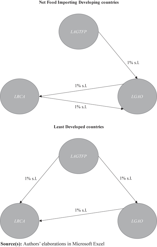
For NFID countries, the credit is capable of stimulating the output, whereas this is not true in the least developed countries (Tables 4 and 5). For both groups of countries, agricultural output has a positive reaction to agricultural productivity but not vice versa. However, it should be considered the connected lending principle, a practice that would undermine the growth and productivity of the country, since financial intermediaries grant loans to some firms based on their special connections rather than on firm characteristics (Dheera-aumpon, 2015; Stiglitz, 2016).
Main results of a PVARs model (Net food importing developing countries)
| Response of | Response to | Statistics | |||
|---|---|---|---|---|---|
| LAGTFP (t−1) | LRCA (t−1) | LGAO (t−1) | R2 RMSE F | F | |
| LAGTFP (t) | 0.7628*** (0.0474) | 0.0165 (0.0142) | 0.0268 (0.0392) | 0.8284 0.0890 197.86 (0.0000) | FLRCA, LGAO 1.13 (0.3245) |
| LRCA (t) | 0.0871 (0.0773) | 0.8873*** (0.0231) | 0.2309*** (0.0639) | 0.9941 0.1452 1131.88 (0.0000) | FLAGTFP, LGAO 8.55*** (0.0002) |
| LGAO (t) | 0.1745*** (0.0473) | 0.0346** (0.0142) | 0.9431*** (0.0392) | 0.9966 0.0889 650.74 (0.0000) | FLAGTFP, LRCA 14.18*** (0.0000) |
| No. of obs. | 422 | ||||
| No. of countries | 29 | ||||
Note(s): ***p < 0.01, **p < 0.05, *p < 0.10. See also notes from Table 1
Source(s): Authors’ calculations
Main results of a PVARs model (Least developed countries)
| Response of | Response to | Statistics | |||
|---|---|---|---|---|---|
| LAGTFP (t−1) | LRCA (t−1) | LGAO (t−1) | R2 RMSE F | F | |
| LAGTFP (t) | 0.8213*** (0.0347) | 0.0480 (0.0908) | 0.0437 (0.0287) | 0.8452 0.0801 273.97 (0.0000) | FLRCA, LGAO 2.04 (0.1309) |
| LRCA (t) | 0.3041*** (0.0932) | 0.8067*** (0.0244) | 0.5713*** (0.0771) | 0.9832 0.2151 1686.23 (0.0000) | FLAGTFP, LGAO 28.66*** (0.0000) |
| LGAO (t) | 0.1341*** (0.0383) | 0.0148 (0.0100) | 0.9259*** (0.0316) | 0.9957 0.0883 1134.49 (0.0000) | FLAGTFP, LRCA 12.78*** (0.0000) |
| No. of obs. | 482 | ||||
| No. of countries | 25 | ||||
Note(s): ***p < 0.01, **p < 0.05, *p < 0.10. See also notes from Table 1
Source(s): Authors’ calculations
In short, the effects of the credit–output–productivity nexus (as emphasized by the statistical significance of the relationships across variables) are stronger for the developing and the OECD countries, and loose for the least developed countries and the NFID countries.
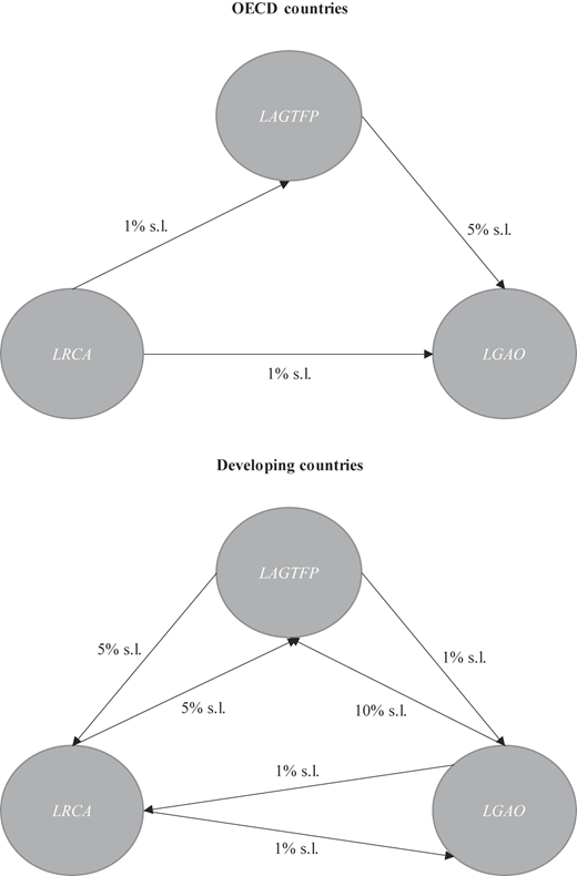
Regarding comparisons with previous results in the literature, the unidirectional causal link from credit access to productivity – found by Rozelle et al. (1999), Feder et al. (1990), Foltz (2004), Guirkinger and Boucher (2008), Dong et al. (2012) and Ali et al. (2014) – is confirmed in the OECD countries subsample (at a 5% significance level) and for the whole sample (at 10%). Moreover, a causal flow running from financial development to economic growth is found only for OECD countries (at 1%), in line with empirical findings provided by King and Levine (1993), De Gregorio and Guidotti (1995), Levine and Zervos (1996), Neusser and Kugler (1998), Rajan and Zingales (1998), Beck et al. (2000), Levine et al. (2000), Rousseau and Wachtel (2000) and Yang and Yi (2008). On the contrary, the opposite direction of causality is established for the full sample and the least developed countries, as in Zang and Kim (2007). Meanwhile, a bidirectional relation between these variables is discovered for developing countries and NFID countries, as shown in Demetriades and Hussein (1996), Demetriades and Luintel (1996), Luintel and Khan (1999), Calderón and Liu (2003) and Hondroyiannis et al. (2005).
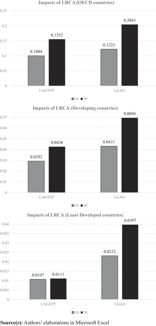
The variance decomposition results (see Table 6 and Figure A2 in the appendix) for our panel allows us to emphasize and comment on the dynamic impacts of the variables ten and twenty periods ahead. Credit access explains at most 4% of the variation of productivity in all but one group: for the OECD countries, credit access explains up to 16% of the variability of productivity (for 20 periods ahead). Similarly, while it is generally true that credit access explains a limited portion (ranging from 2% to 7%) of the variability of the output, for the OECD countries and the NFID, the shares are considerably larger (up to 20%). Again, the impacts increase over time. Another aspect of relevance is that while the variance decomposition of credit access is mainly due to its own variation for the OECD countries (around 93%), this is not true for developing, the least developed and, above all, NFID countries: predictions 20 periods ahead highlight that these shares are equal to 71% for developing countries and 75% for the NFID countries. Moreover, agricultural output contributes in a remarkable and increasing way to the variability of credit access, the only exception being OECD countries. After 20 periods, LRCA variability is explained by variation in LGAO for 26% in developing countries, 19% in NFID and 47% in the least developed. However, the opposite seems true only for OECD countries, where after 20 periods credit access explains the variability of the agricultural output up to 20%.
Variance decompositions
| Variable | LAGTFP | LRCA | LGAO |
|---|---|---|---|
| Full sample (10 periods ahead) | |||
| LAGTFP | 0.9484 | 0.0366 | 0.0150 |
| LRCA | 0.0287 | 0.8762 | 0.0951 |
| LGAO | 0.4262 | 0.0565 | 0.5173 |
| Full sample (20 periods ahead) | |||
| LAGTFP | 0.9418 | 0.0426 | 0.0156 |
| LRCA | 0.0325 | 0.7708 | 0.1967 |
| LGAO | 0.3451 | 0.0923 | 0.5626 |
| OECD (10 periods ahead) | |||
| LAGTFP | 0.8886 | 0.1004 | 0.0110 |
| LRCA | 0.0430 | 0.9391 | 0.0179 |
| LGAO | 0.4662 | 0.1223 | 0.4115 |
| OECD (20 periods ahead) | |||
| LAGTFP | 0.8332 | 0.1552 | 0.0116 |
| LRCA | 0.0512 | 0.9252 | 0.0236 |
| LGAO | 0.4150 | 0.2043 | 0.3807 |
| Developing (10 periods ahead) | |||
| LAGTFP | 0.9481 | 0.0292 | 0.0227 |
| LRCA | 0.0343 | 0.8443 | 0.1214 |
| LGAO | 0.4207 | 0.0431 | 0.5362 |
| Developing (20 periods ahead) | |||
| LAGTFP | 0.9344 | 0.0426 | 0.0230 |
| LRCA | 0.0357 | 0.7090 | 0.2553 |
| LGAO | 0.3284 | 0.0694 | 0.6022 |
| Net food importing developing (10 periods ahead) | |||
| LAGTFP | 0.9579 | 0.0317 | 0.0104 |
| LRCA | 0.0598 | 0.8621 | 0.0781 |
| LGAO | 0.5508 | 0.0647 | 0.3845 |
| Net food importing developing (20 periods ahead) | |||
| LAGTFP | 0.9461 | 0.0400 | 0.0139 |
| LRCA | 0.0622 | 0.7457 | 0.1921 |
| LGAO | 0.4044 | 0.1348 | 0.4608 |
| Least developed (10 periods ahead) | |||
| LAGTFP | 0.9568 | 0.0107 | 0.0325 |
| LRCA | 0.0523 | 0.6980 | 0.2497 |
| LGAO | 0.5157 | 0.0232 | 0.4611 |
| Least developed (20 periods ahead) | |||
| LAGTFP | 0.9396 | 0.0111 | 0.0493 |
| LRCA | 0.0501 | 0.4809 | 0.4690 |
| LGAO | 0.3829 | 0.0397 | 0.5774 |
Note(s): Percent of variation in the row variable explained by column variable
Source(s): Authors’ calculations
The graphical representation of the contribution of credit on productivity and output is quite different across groups of countries. In particular, the impacts are considerable for OECD countries both in the short period (about 10–12%, 10 years ahead) and in the long period (about 15–20%, 20 years ahead), whereas they are very limited (6% at most) for developing (always below 4%) and the least developed countries (always below 4%). Additionally, while the contribution of credit access to productivity and output is largely increasing over time for OECD countries (respectively +5% or +8%, moving from 10 periods ahead to 20 periods ahead), the increase is (in absolute terms) very modest for developing and the least developed countries (Figure A2). Put differently, credit access seems to have a stronger (and longer-term) effect on agricultural development only for countries with a relatively higher level of economic development (i.e., high GDP), whereas its contribution is weaker (and shorter term) for countries with a relatively lower level of economic development. Figure A1 in the appendix gives a graphical representation of the results of the causality analysis.
As regard the macroeconomic literature, such results are in line with those of King and Levine (1993) and De Gregorio and Guidotti (1995) for 80 countries, Levine et al. (2000) for 74 economies, Yang and Yi (2008) for Korea, Pradhan et al. (2016) for 18 EU countries and Asteriou and Spanos (2019) for 26 EU countries, as they all revealed the existence of a unidirectional causal link running from financial development to economic output, without feedback. Nonetheless, our findings contradict those of Mtar and Belazreg (2021) since they supplied evidence of a reverse causal direction for 27 OECD countries. Finally, our evidence does contrast with Cheng et al. (2021) and Siddikee and Rahman (2021) since both studies revealed a negative estimated coefficient related to financial development. Shifting to the micro-based literature, the present results extend the conclusion drawn in a range of cross-section and panel assessments based on firm-level series, notably Feder et al. (1990) and Dong et al. (2012) for China, Foltz (2004) for Tunisia, Hartarska et al. (2015) and Sabasi et al. (2020) for the United States, Aghion et al. (2019) for France, Issahaku et al. (2020) for Ghana, Rodríguez-Pose et al. (2021) for 11 EU countries, and which unanimously demonstrated that credit access triggers productivity, which, in turn, determines the growth of aggregate output.
Besides, our results also echo those of Shahbaz et al. (2013) and Yazdi and Khanalizadeh (2014) as they both underlined that financial development and agricultural output improve each other in Pakistan and Iran, respectively. Furthermore, they partially confirm the findings of Zakaria et al. (2019), who revealed the existence of a non-linear U-shaped relationship between financial development and productivity in the agricultural sector of five Asian countries. Finally, our insights are not in line with Olowu et al. (2019), as they showed that financial development and agricultural value-added reduce employment in 11 African countries, whereas Farooq et al. (2021) stressed the existence of a one-way causality between credit access and agricultural output reduction. Compared with the micro-based literature, the above results agree with Petrick (2004) for Poland, Alfaro et al. (2009) for 72 countries, Nakano and Magezi (2020) for Tanzania, and Agbodji and Johnson (2021) for Togo, since these studies failed to find empirical support to the existence of a significant causal effect of credit access on productivity.
4. Conclusions and policy implications
The relationship among financial development, productivity and growth has been extensively examined in the literature. However, the nature and directions of these linkages remain unclear, and it is still debated. We investigate these relationships. We have also analyzed how the triad credit–outcome–productivity differs across income groups. The study has been conducted on an illustrative sample of 130 countries, divided into four subgroups, using FEVDs and PVAR methods.
Time-series outputs unanimously show that productivity is stimulated by credit access, and the latter is facilitated by higher levels of agricultural output. Put differently, higher levels of output stimulate economic development in the agricultural sector via the productivity channel and, more importantly, by improving credit access (although the size of this effect tends to be larger for high-income countries). These results, specific to the agricultural sector, are in line with the arguments supported by Levine et al. (2000) and Beck et al. (2000) on the positive relationship between credit markets development and economic growth, and the role of productivity growth. Moreover, the discovered relationships among credit, output and productivity are in line with earlier and recent studies (Guirkinger and Boucher, 2008). It is interesting to note that Verdoorn’s law (Verdoorn, 1949) is confirmed in all our estimates: in fact, output significantly influences productivity in all tested samples.
Notably, the fundamentals of the agricultural economy follow different mechanisms across countries: the relationships among the three variables are tighter (and of longer impact) for OECD countries, where credit stimulates both productivity and output. On the other hand, these relationships are loose (and of the shorter term) in developing countries, where the stimulus to agricultural output is mainly from productivity. A plausible explanation of our findings is provided by the well-established literature on the role of technological innovations in agriculture (Foster and Rosenzweig, 1995; Conley and Udry, 2010). The role of credit is more important for developed economies, and advanced agricultural sectors where agricultural firms may easily exploit, through credit, the advantages of technological innovations. Providing credit to firms located in developing countries can only boost production because technologies spread slowly through learning-by-doing and learning-from-other mechanisms, and the gains from advanced technologies cannot be exploited quickly. Accordingly, in developing countries, credit access tends to significantly affect production, whereas in developed countries, it also substantially impacts productivity.
The credit–output–productivity nexus is stronger for the developing countries, followed by OECD countries, and weaker for the least developed countries (LDC) and the NFID.
Our results favor the motivations for intervention in credit markets as a strategy to promote economic development. Following the argument of Bardhan and Udry (1999), who stated that “agricultural credit was conceptualized as factor of production, […] an increase in supply of credit would lead to an increase in production and income,” we conclude that policies facilitating credit access leverage output. In addition, the evidence on the developed economies suggests that such policies may affect both production and productivity. A direct implication of our analysis is that, while it is true that credit constraints tend to limit growth (Azariadis and Drazen, 1990), the higher the economic development, the more agricultural development is hampered by a lack of credit access. Put differently, pro-growth policy interventions in the least developed countries may not necessarily require the development of credit markets, whereas the opposite would be true in developed economies.
A caveat of this analysis is that we are not able to disentangle the mechanisms that trigger the reciprocal causality between credit and productivity. However, by observing that this link is clearly connected to the level of economic development, we attempt to open a constructive research caveat about the existence of potential synergies among these variables, which should be further investigated to enhance our understanding of how the agricultural sector evolves and responds to endogenous drivers. Further inspecting the heterogeneous nature of the impacts of policies devoted to productivity and credit access across sectors in developing countries is no longer avoidable. On this matter, the use, replication and extension of data-intensive methods (e.g. machine learning experiments and wavelet analysis) in complement to advanced econometric procedures may emerge as a potentially fruitful direction (Magazzino et al., 2021b; Mele et al., 2021).
Notes
Briefly speaking, it states that in the long-run productivity generally grows proportionally to the square root of output.
We do not rely on a theoretical framework, but rather refer to the literature on panel data to emphasize the dynamic links across variables.
See, for more details: https://www.ers.usda.gov and https://www.fao.org/faostat.
In practice, the literature suggests the following procedure: randomly generating a draw of Φ coefficients for model (1) by using the coefficients previously estimated and their associated variance-covariance matrix, before re-calculating the impulse-responses. This procedure is then repeated 1,000 times. Finally, the 5th and 95th percentiles of this distribution are generated and used to construct the 95% confidence interval for the impulse-responses.
Other classifications (e.g. the dichotomous classification of countries in developed and developing countries) are nested in the SCG classification.

