
To enhance portfolio decision-making using a capital asset pricing model-based clustering analysis.
Capital asset pricing model (CAPM); K-means clustering; agglomerative clustering.
Employing clustering along with CAPM to identify varying levels of risk appetite among customers enables the customization of security recommendations, enhancing client satisfaction and portfolio performance.
By employing multi-factor models as the foundation for clustering, thereby integrating additional dimensions of risk and return.
1. Introduction
The emergence of the Capital Asset Pricing Model (CAPM) by Sharpe (1964) and Lintner (1965) marked a pivotal moment in asset pricing theory, building upon the foundational work of Harry Markowitz on diversification and modern portfolio theory (Markowitz, 1991). This model fundamentally posits that not all risks should influence asset prices and offers insights into the relationship between risk and return (Rossi, 2016). Before the advent of the CAPM, risk was not accorded significant consideration in the computation of capital costs. The CAPM revolutionized this perspective by providing a framework to translate risk into expected returns on investments. Nevertheless, its application has engendered ongoing debate, with critics often highlighting its reliance on assumptions that may not fully align with real-world conditions (Rossi, 2016). Despite these criticisms, the CAPM remains widely employed across various domains even 4 decades after its inception. Its utility extends to assessing expected returns on stocks, conducting merger and acquisition analyses, capital budgeting, and evaluating warrants and convertible securities. Given the perceived complexity of capital markets, retail investor engagement has been limited, with only a minority participating in equity markets, and retail involvement growing incrementally (Chakri et al., 2023). However, the democratization of artificial intelligence and increased access to high-quality data present opportunities for machine learning models to navigate these intricate markets, potentially enhancing retail engagement. Chen and Zhou (2023) delve into the motivations for applying machine learning (ML) to equity investing, underscoring the transformative potential of these technologies in augmenting decision-making processes within capital markets.
A significant portion of current literature delves into harnessing ML techniques for forecasting various asset prices, often juxtaposing the efficacy and precision of ML tools against traditional econometric models. For instance, Khoa and Huynh (2023) undertook a comparative analysis between the CAPM and the Fama-French three-factor model (Fama and French, 1996) using specific ML methodologies. Simonian et al. (2019) addressed the limitations of linear factor models by leveraging ML algorithms to enhance traditional modeling approaches. Despite these advancements, there remains a dearth of studies investigating the integration of the CAPM with clustering methodologies. This study endeavors to fill this void by examining the synergy between the CAPM framework and clustering approaches, aiming to shed light on their potential synergies and implications for asset pricing and predictive modeling.
Clustering analysis, an unsupervised machine learning technique, is designed to discern natural groupings within a dataset by assessing similarities between data points. The underlying principle involves partitioning data points into clusters in a manner that ensures points within the same cluster are more akin to each other than to those in other clusters. In financial research, one of the key applications of clustering analysis is the delineation of market segments. Through clustering assets based on historical returns, volatility, correlations, and other pertinent metrics, researchers can unearth distinct market segments characterized by unique attributes. Furthermore, clustering analysis serves as a valuable tool for grouping assets with analogous risk profiles. By clustering assets according to their risk-return characteristics, such as beta within the framework of the CAPM, investors can pinpoint assets that tend to exhibit concurrent movements in response to market fluctuations. This categorization facilitates the construction of diversified portfolios by selecting assets from disparate clusters, thereby mitigating concentration risk, and enhancing portfolio resilience.
Our study focuses on examining how S&P Top 50 stocks cluster based on their risk and expected return profiles, as captured by a range of financial and ESG metrics. To achieve this objective, we adopt a comprehensive approach akin to that of Nanda et al. (2010), which integrates financial modeling, feature engineering, and machine learning methodologies. Specifically, leveraging the well-established theoretical underpinnings of the CAPM, we compute the expected returns of the S&P top 50 stocks over the past decade. Subsequently, our study endeavors to explore the potential of unsupervised machine learning techniques, particularly the K-means and agglomerative clustering algorithms. These algorithms are employed in conjunction with the CAPM-derived expected returns and other pertinent financial and sustainability metrics as parameters within a guided clustering framework. Through this approach, our study aims to make several key contributions to the field, including:
Our study adopts a multidimensional approach by integrating financial modeling, specifically the CAPM, with clustering algorithms. This innovative combination extends beyond traditional clustering analyses, offering a novel methodology for analyzing stock data.
By clustering stocks based on features derived from the CAPM, our study aims to reveal diverse risk-return profiles. This approach provides potential investors with a fresh perspective on how various stocks converge, enabling them to make more informed investment decisions.
The utilization of clustering methods facilitates the identification of hidden patterns and trends within financial data. By transforming these insights into actionable information, our analysis provides valuable guidance for financial practitioners seeking to optimize their investment strategies.
Our analysis considers ESG scores alongside CAPM metrics, offering a comprehensive understanding of how sustainability factors influence asset clustering. This integration enhances risk management practices and ensures that investments align with ethical values. Moreover, incorporating ESG criteria promotes long-term performance and facilitates compliance with regulatory standards. Additionally, it enhances portfolio diversification by identifying sustainable assets with potential for long-term growth.
The findings of the study demonstrate that both clustering approaches yield highly similar cluster profiles, with two principal components accounting for 44% of the variance in the data. Examination of these cluster profiles provides valuable insights into how stocks can be grouped to optimize diversification and minimize risk, offering significant benefits for both portfolio managers and retail investors.
The remainder of the paper is structured as follows: Section 2 presents a comprehensive review of the relevant literature. Following this, Section 3 elucidates the theoretical framework underpinning the study. In Section 4, we delineate the data sources utilized and the preprocessing steps undertaken. Section 5 expounds upon the clustering algorithms employed and outlines the methodology adopted in this study. Subsequently, Section 6 delves into the findings of the cluster analysis, accompanied by a discussion of their implications. Finally, Section 7 concludes the paper by providing insights into the limitations of the study and offering directions for future research endeavors.
2. Literature review
Traditional ML methods have seen extensive use in financial innovation and asset pricing, as evidenced by studies conducted by Maiti et al. (2020), Vaidyanathan et al. (2023), Das et al. (2023), Rajendran et al. (2024), and Ranjan et al. (2023). As technological advancements continue, an increasing number of investors and financial researchers are integrating traditional financial theoretical frameworks with machine learning techniques to better navigate the complexities of asset pricing. In the financial domain, investors grapple with a deluge of information sourced from diverse channels (Nagel, 2021). Within such data-rich environments, the evolving field of machine learning emerges as a promising toolkit for effectively addressing predictive challenges (Nagel, 2021). Researchers have found ML techniques, such as neural networks and random forests, to be invaluable for identifying potential winners and losers in financial markets. For instance, Ndikum’s (2020) study utilized state-of-the-art ML techniques and high-performance computing infrastructures to conduct a comprehensive evaluation. The findings demonstrated the superior predictive performance of machine learning algorithms over the CAPM framework. Leveraging approximately 200-time series features, ML algorithms exhibited greater flexibility in forecasting annual returns for individual US equities. As we transition into the era of big data, the capacity of machine learning techniques to process vast datasets and extract meaningful insights will continue to revolutionize the finance sector. This paradigm shift underscores the necessity for innovative methodologies, such as CAPM-based clustering analysis, to harness the strengths of both traditional finance theories and cutting-edge data-driven approaches.
Lewellen (2015) employs cross-sectional regressions incorporating 15 firm characteristic variables, such as size and momentum, with considerable effectiveness in forecasting future monthly returns. Numerous studies, including Subrahmanyam (2010), have illustrated the feasibility of capturing a significant portion of the variance in cross-sectional stock returns through modeling the information embedded in firm characteristics. Gu et al. (2020) synthesize the empirical asset pricing literature with the realm of machine learning, emphasizing that machine learning accommodates a broader array of potential predictor variables and more flexible functional specifications compared to conventional empirical methods in asset pricing. This flexibility enables researchers to expand the frontier of risk premium measurement. Gu et al. (2020) elucidate that the asset pricing literature encompasses myriad stock-specific predictive factors, numbering in the hundreds, alongside dozens of macroeconomic indicators for the broader market. Moreover, many of these predictors exhibit robust correlations and similarities. Traditional prediction methodologies encounter challenges when the number of predictors approaches or surpasses the number of observations, or when predictors demonstrate high correlations. ML techniques, with their emphasis on feature engineering and dimensionality reduction, provide a well-suited approach to address such intricate prediction challenges. By curtailing the degrees of freedom and consolidating redundant variation among predictors, machine learning methods effectively handle these complexities (Gu et al., 2020).
Wu et al. (2022) utilize the k-means clustering algorithm to segment stocks, delineate distinct pools of stock types, and refine return calculations for the Sharpe ratio. They consider the continuous trend characteristics of the market to mitigate downside risk. Additionally, the authors integrate inverse volatility weighting, risk parity, and Markowitz’s portfolio theories to compute the necessary weights. Through experimentation, they determine the optimal number of stocks for the portfolio. The outcomes are then validated through both statistical analysis and experimental results, thereby establishing the effectiveness of their proposed methodology. Similarly, Tekin and Gümüş (2017) incorporate financial indicators such as price/earnings ratio, market value/book value ratio, dividend yield, return on assets, return on equity, and other return and risk measures as variables in their clustering analysis of 88 stocks in the Borsa Istanbul 100 Index. Furthermore, Nanda et al. (2010) adopted a similar approach, utilizing valuation ratios as variables in k-means and fuzzy c means algorithms to cluster stocks from the Bombay Stock Exchange.
Recent literature has increasingly integrated sustainability themes into analyses, reflecting the growing recognition of the material financial implications associated with sustainability metrics (Maiti, 2021). Kaminskyi and Nehrey (2023) exemplify this trend by adopting a cluster approach to portfolio management, incorporating sustainability into their clustering algorithms for the constituents of the German market DAX index. They utilize ESG scores as a proxy for sustainability alongside conventional investment indicators, thereby offering a more comprehensive approach to clustering analyses compared to earlier studies. In a similar vein, several studies, including Xu et al. (2020), employ two-stage fusion models using technical indicators as variables. They find that k-means clustering on these variables can enhance the prediction accuracy of fusion models. Building upon this literature, our study takes a unique approach by combining technical indicators and sustainability metrics, in addition to CAPM-derived results, for the S&P Top 50. This novel approach merges financial modeling with clustering algorithms, offering a distinctive perspective on asset pricing. By uncovering diverse risk-return profiles and revealing hidden patterns within financial data, our study provides actionable insights for portfolio management. Moreover, the integration of ESG criteria enhances risk management and aligns investments with ethical values, further contributing to the broader discourse on sustainable finance.
3. Theoretical framework
The Capital Asset Pricing Model (CAPM) was initially formulated in the early 1960s by William Sharpe, marking a seminal advancement in financial modeling and asset pricing (Sharpe, 1964). As described by Lewinson (2020), the CAPM elucidates the connection between the anticipated return on a risky asset and the market risk, commonly referred to as systematic or undiversifiable risk.
Mathematically, it is expressed in Equation (1).
Where, = Expected return on asset i, Beta coefficient of asset i, Expected Market return, and Risk free rate. The beta coefficient captures the sensitivity of asset i’s returns with respect to the market return and its potential values are interpreted below (Lewinson, 2020).
If <= −1: The asset moves in the opposite direction as the benchmark and in a greater magnitude than the negative of the benchmark.
If −1 < < 0: The asset moves in the opposite direction to the benchmark.
If = 0: There is no correlation between the asset’s price movement and market benchmark.
If 0 < < 1: The asset moves in the same direction as the market, but by a smaller magnitude.
If = 1: The asset and the market are moving in the same direction by the same magnitude.
If > 1: The asset moves in the same direction as the market, but by a greater magnitude.
is calculated as the ratio of the covariance between expected returns on the asset and the market, divided by the variance of expected returns on the market, as expressed in Equation (2).
, are then plugged into the CAPM, to estimate the expected asset return ().
4. Data and variables
4.1 Variables and data sources
4.1.1 CAPM variables
The S&P 500 Top 50 comprises the 50 largest companies within the S&P 500 index, serving as a reflection of US mega-cap performance. In our study, these Top 50 securities are selected as assets, with the S&P 500 index serving as the market benchmark. Subsequently, we acquire adjusted closing price data spanning from December 31, 2013, to December 31, 2023, sourced from Yahoo Finance. Additionally, we incorporate a non-zero risk-free rate using the 13-week (3-month) Treasury Bill, accessed via the Yahoo Finance website.
4.1.2 Clustering variables
Subsequently, a dataset is constructed for the selected sample. The outputs derived from the CAPM, specifically the expected returns for each of the Top 50 stocks, are utilized as one of the variables. Additionally, other pertinent variables are incorporated, as outlined in Table 1. The data for the variables are primarily sourced from Yahoo Finance, while the ESG scores and categories are obtained from Morningstar Sustainalytics. These variables encompass essential financial indicators commonly utilized in fundamental analysis (Momeni et al., 2015), thereby offering insights into the risks associated with the underlying assets.
Data dictionary
| Variable | Data type | Description |
|---|---|---|
| Ticker | Object | Ticker Symbol |
| Security | Object | Company Name |
| GICS Sector | Object | Economic sector assigned by GICS basis business operations |
| 52 Week Price Change | Float64 | Percentage change in the stock price in 52 weeks |
| ESG Scorea | Float64 | Measures absolute ESG risk |
| ESG Risk Cat | Object | Qualitative classification of ESG risk |
| ROE | Float64 | Net income by shareholders’ equity (TTM) |
| Current Ratio | Float64 | Current assets by current liabilities (MRQ) |
| Free Cash Flow | Int64 | Measured in thousands (TTM) |
| Net Income Avi to Common | Float64 | Measured in Billion USD |
| Diluted EPS | Float64 | Net income minus preferred dividend by shares outstanding (TTM) |
| Market Cap | Float64 | Total market value of outstanding shares measured in Billion USD |
| Forward P/E | Float64 | Current share price by estimated future earnings per share |
| PEG (5 yr exp) | Float64 | Stock price to earnings ratio divided by the growth rate of its earnings |
| P/B | Float64 | Price per share to book value per share (MRQ) |
Note(s): GICS = Global Industry Classification Standard; ESG = Environmental, Social, and Governance; MRQ = Most Recent Quarter; TTM = Trailing Twelve Months
aSustainalytics’ ESG Risk Ratings measure a company’s exposure to industry-specific material ESG risks and how well a company is managing those risks. Five categories are used to assess potential impacts on a company’s enterprise value. The risk rating scale classifies risks into five categories: Negligible, Low, Medium, High, and Severe, based on specific numerical ranges (0–10, 10 to 20, 20 to 30, 30 to 40, 40 to 50)
Source(s): Authors’ own work
4.2 Data preprocessing
4.2.1 Dealing with missing values
Missing “Nan” values for the financial indicators are populated using data from secondary sources like news articles. There are no duplicate values in the dataset.
4.2.2 Outliers
Outliers have been identified within the dataset; however, they have not been addressed and are presumed to represent genuine data points rather than anomalies (Vaidyanathan et al., 2023).
4.2.3 Feature engineering (scalar transformation)
Following the removal of non-numerical columns from the dataset (GICS Sector, Security, and ESG Risk Category), the data is scaled using the 'StandardScaler' from scikit-learn. Specifically, the “fit_transform” method is utilized, involving fitting the scaler on the data and subsequently transforming it (VanderPlas, 2016). This methodology is selected to standardize the data based on the mean and standard deviation of the training data. Such standardization is a common practice in machine learning to ensure uniform scaling of features and mitigate bias.
5. Methodology
5.1 Implementing the CAPM
For the selected decade, only the last available price per month is retained, and the monthly returns are calculated as the percentage change between subsequent observations. The betas for the respective stocks are estimated using the covariance approach. Subsequently, the risk-free rate ( is computed to accommodate a non-zero risk-free rate, although assuming a zero is reasonable. The risk-free return, expressed as daily values, is converted to monthly values, and illustrated in Figure 1.
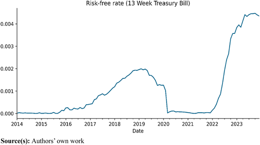
The current of 0.004% is employed for further calculations. Additionally, the is calculated similarly using ˆGSPC data (proxied by the S&P500) and is determined to be 10.66%. Finally, these values, along with the respective stock Betas, are incorporated into the CAPM equation to derive the expected returns for each of the stocks. Subsequently, an exploratory data analysis is conducted.
5.2 Model selection
In our model, we adopt a supervised approach to the common unsupervised clustering algorithms using labeled data. This approach is valid in this scenario since the dataset contains predefined financial metrics that help guide the formation of clusters. This facilitates a more guided exploration of the underlying patterns in the dataset. In this study, we adopt and evaluate the K-means and agglomerative clustering methods. These methods are ideal for homogeneous metric-based clustering and multidimensional data. Moreover, they are relatively straightforward to interpret, making them better suited for the target audience, which includes retail investors and financial analysts who may not possess advanced machine learning expertise.
5.3 K-means clustering
The K-means algorithm aims to partition the dataset into “K” distinct, non-overlapping clusters. This process iteratively assigns data points to the nearest cluster centroid and updates the centroids based on the mean of the assigned points. Iterations continue until convergence, stabilizing the assignments and centroids. The algorithm minimizes inter-cluster variance, ensuring each cluster is as compact and separated as possible (Das et al., 2023).
5.3.1 Determining the number of clusters
The elbow method serves as a valuable tool in determining the optimal value of “K” in K-means clustering. This technique identifies a point where the rate of decrease in distortion, represented by the average distance of points to their assigned centroid, begins to decelerate, forming an “elbow” in the plot. This point signifies a favorable balance between capturing variance in the data and avoiding overfitting. Concurrently, the silhouette score emerges as a pivotal metric for evaluating the quality of clustering. This score quantifies how similar an object is to its own cluster (cohesion) relative to other clusters (separation), spanning a range from −1 to 1. A higher silhouette score indicates a stronger alignment of the object with its designated cluster and a weaker alignment with alternative clusters. In practice, we implement a code that iterates across a range of cluster numbers, fitting a K-means model for each iteration and computing the corresponding silhouette score. These scores are then aggregated into a “sil_score list,” and the results are printed iteratively. Subsequently, a plot of silhouette scores against the number of clusters aids in identifying the optimal number. This is determined by selecting the number of clusters associated with the highest silhouette score. Given the sensitivity of K-means performance to the initial placement of centroids, we conduct iterative runs and average the silhouette scores to enhance the robustness of our evaluation. This iterative approach ensures a more stable and consistent assessment of clustering results, thereby bolstering the reliability of our findings.
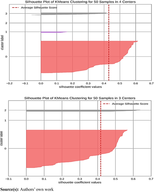
In addition to employing the elbow method, we integrate the silhouette coefficient approach to ascertain the optimal number of clusters. While the silhouette coefficient evaluates the suitability of individual data points to their assigned clusters, offering a local measure of cluster cohesion, the silhouette score provides a global assessment of overall cluster quality and distinctiveness by averaging these coefficients. Upon determining the optimal number of clusters through the silhouette score, we execute the K-means algorithm using this specified number of clusters. Subsequently, we derive the cluster profiles, unveiling the distinctive characteristics and patterns inherent within each cluster. This comprehensive approach enables a nuanced understanding of the underlying structure of the dataset, facilitating informed decision-making processes.
5.4 Agglomerative clustering
Agglomerative clustering, a variant of hierarchical clustering, initially treats each data point as an individual cluster. Subsequently, it iteratively merges pairs of clusters based on their proximity. Specifically, it calculates the distance between every pair of clusters and progressively amalgamates the closest clusters (Jaroonchokanan et al., 2022). This merging process continues until a termination criterion is satisfied. Consequently, a dendrogram, a hierarchical tree-like structure is formed, illustrating the clustering hierarchy and the relationships between clusters. This approach offers insights into the inherent structure of the dataset and facilitates the identification of meaningful cluster formations.
5.4.1 Distance metrics and linkage methods
In our analysis, we employ several distance metrics, including “euclidean,” “chebyshev,” “mahalanobis,” and “cityblock,” to quantify the dissimilarity between data points. Additionally, we utilize various linkage methods, such as “single,” “complete,” “average,” “centroid,” “ward,” and “weighted,” to determine the inter-cluster distance. These diverse metrics and methods offer flexibility in capturing different aspects of data dissimilarity and cluster formation, allowing for a comprehensive exploration of clustering structures within the dataset.
5.4.2 Cophenetic correlation calculation
For each pairing of distance metric and linkage method, we conduct hierarchical clustering utilizing the linkage function from “scipy.cluster.hierarchy.” Following this, we estimate the cophenetic correlation coefficient using the “cophenet” function, which offers crucial insights into the fidelity of the hierarchical clustering results. Our primary objective is to pinpoint the combination that produces the highest cophenetic correlation, signifying a more robust depiction of the underlying data structure. Subsequently, we extract the cluster profiles and juxtapose them with those derived from the K-means algorithm to discern any notable disparities or similarities in clustering outcomes.
5.5 Understanding the cluster agreement
Initially, we examine the labels assigned by both the K-means and hierarchical clustering techniques to each security. Subsequently, we employ Cohen’s Kappa to gauge the consistency between the labels generated by the two methods. Additionally, we utilize the Adjusted Rand Index to gain deeper insights into the clustering outcomes and their agreement.
5.6 Principal component analysis
Finally, Principal Component Analysis (PCA) is employed to reduce the dimensionality of the dataset to two principal components, enabling visualization of the clusters and elucidating the explained variance of these components. This simplified representation aids in obtaining a clearer comprehension of the clustering outcomes and extracting actionable insights from the data.
6. Results and discussion
6.1 CAPM results
The outcomes of this model are succinctly summarized in Table 2 and are subsequently utilized in the preliminary exploratory data analysis.
CAPM results
| Ticker | Sector | Rank | Beta | Expected returns (annual %) |
|---|---|---|---|---|
| DHR | Healthcare | 1 | 0.89 | 9.51 |
| TMO | Healthcare | 2 | 0.88 | 9.41 |
| ABT | Healthcare | 3 | 0.86 | 9.17 |
| ABBV | Healthcare | 4 | 0.74 | 7.91 |
| PFE | Healthcare | 5 | 0.66 | 7.01 |
| UNH | Healthcare | 6 | 0.63 | 6.75 |
| JNJ | Healthcare | 7 | 0.58 | 6.18 |
| BMY | Healthcare | 8 | 0.51 | 5.47 |
| MRK | Healthcare | 9 | 0.43 | 4.62 |
| LLY | Healthcare | 10 | 0.32 | 3.51 |
| AMD | IT | 1 | 2.12 | 22.54 |
| NVDA | IT | 2 | 1.75 | 18.57 |
| QCOM | IT | 3 | 1.36 | 14.46 |
| AAPL | IT | 4 | 1.28 | 13.64 |
| ADBE | IT | 5 | 1.28 | 13.59 |
| CRM | IT | 6 | 1.27 | 13.56 |
| ACN | IT | 7 | 1.18 | 12.59 |
| AVGO | IT | 8 | 1.09 | 11.58 |
| TXN | IT | 9 | 1.07 | 11.45 |
| ORCL | IT | 10 | 1.04 | 11.08 |
| MSFT | IT | 11 | 0.97 | 10.35 |
| CSCO | IT | 12 | 0.96 | 10.25 |
| INTC | IT | 13 | 0.95 | 10.09 |
| DIS | Communication | 1 | 1.26 | 13.47 |
| NFLX | Communication | 2 | 1.22 | 13.01 |
| META | Communication | 3 | 1.06 | 11.28 |
| GOOGL | Communication | 4 | 1.04 | 11.11 |
| CMCSA | Communication | 5 | 1.00 | 10.69 |
| VZ | Communication | 6 | 0.43 | 4.63 |
| TSLA | Consumer | 1 | 1.89 | 20.14 |
| AMZN | Consumer | 2 | 1.28 | 13.62 |
| HD | Consumer | 3 | 1.02 | 10.88 |
| NKE | Consumer | 4 | 1.00 | 10.65 |
| MCD | Consumer | 5 | 0.67 | 7.19 |
| KVUE | Consumer Staples | 1 | 1.98 | 21.08 |
| COST | Consumer Staples | 2 | 0.83 | 8.82 |
| KO | Consumer Staples | 3 | 0.58 | 6.26 |
| PEP | Consumer Staples | 4 | 0.57 | 6.08 |
| WMT | Consumer Staples | 5 | 0.45 | 4.84 |
| PG | Consumer Staples | 6 | 0.44 | 4.68 |
| CVX | Energy | 1 | 1.12 | 11.91 |
| XOM | Energy | 2 | 0.97 | 10.35 |
| BAC | Financials | 1 | 1.38 | 14.72 |
| WFC | Financials | 2 | 1.15 | 12.29 |
| JPM | Financials | 3 | 1.13 | 12.08 |
| MA | Financials | 4 | 1.10 | 11.74 |
| V | Financials | 5 | 0.97 | 10.38 |
| BRK | Financials | 6 | 2.61 | −27.6 |
| LIN | Materials | 1 | 0.89 | 9.46 |
| NEE | Utilities | 1 | 0.43 | 4.65 |
Source(s): Authors’ own work
6.1.1 Sectoral analysis of expected returns and beta values
The analysis of expected returns and beta values reveals clear distinctions across sectors, reflecting different risk-return profiles. The Information Technology (IT) and Consumer Discretionary (mentioned as “Consumer” in Table 2) sectors exhibit high expected returns accompanied by high beta values, indicating these sectors are attractive for growth-oriented investors but come with greater market risk. Conversely, Consumer Staples and Utilities show lower expected returns and low beta values, aligning with their reputation as defensive sectors that offer stability to market fluctuations. The Financials sector presents mixed results, with some stocks like Bank of America showing moderate returns and risk, whereas others, such as Berkshire Hathaway, display high beta with negative returns, reflecting sectoral sensitivity to economic cycles. These observations emphasize the trade-off between risk and return across sectors.
6.2 Results from exploratory data analysis
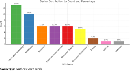
Utilizing the CAPM expected returns as a feature alongside other fundamental ratios in the final dataset comprising 50 rows and 16 columns, we observe the following statistical insights. Among the 11 unique GICS sectors, Information Technology emerges as the most prevalent (Refer to Figure 2).
The average expected returns stand at 9.83% with a median of 10.51%, suggesting a right skew in the distribution. Notably, the average 52-week price change is 24.5%, accompanied by a substantial standard deviation of 45.5%, indicating considerable variability. Market capitalization displays a wide range of $3000 billion. In terms of Return on Equity (RoE), the mean is 115.86, while the median is 23.63, signaling the presence of significant positive outliers and a right-skewed distribution. Similarly, diluted EPS exhibits a pronounced right skew, with a median of $6 and a mean of $1061, suggestive of extreme positive outliers. Although the average Price to Book and Price to Earnings ratios are positive, indicating a lack of distressed stocks on average, the minimum Price to Book ratio is negative, possibly indicating financial stress in at least one observation where liabilities exceed assets. The mean ESG score is 21.25, closely aligned with the median of 20.35, suggesting few outliers in this aspect. Additionally, nearly half of the sample falls under the low-risk category.
6.2.1 Univariate analysis
Figure 3 provides a comprehensive visualization of key statistical features of financial and performance metrics. The central tendency of the data is represented by the box in the plot, indicating the interquartile range (IQR) delineated by the first (Q1) and third (Q3) quartiles, with the median (Q2) depicted by a line within the box. Dispersion is illustrated by the length of the whiskers extending from the box, signifying the variability of data points beyond the IQR. Outliers, depicted as individual data points beyond the whiskers, are identified for further scrutiny. Skewness of the distribution is inferred from the asymmetry of the boxplots; if the median is closer to one end of the box, it suggests skewness in that direction. Additionally, when coupled with histograms, boxplots assist in evaluating the overall shape of the distribution, revealing that many distributions appear to be non-normal.
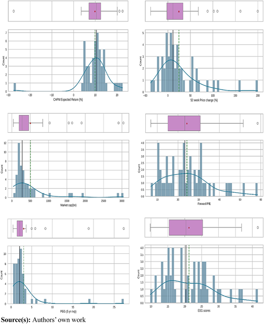
Moreover, these variables offer critical insights into company specific idiosyncrasies. The CAPM expected returns exhibit a wide range, with significant outliers on both the positive and negative sides. The central tendency, as shown by the boxplot, shows that most stocks have returns clustered around the 10% mark, though extreme values suggest considerable variability in market expectations. The 52-week price change distribution shows a strong right skew, indicating that while many stocks experienced moderate growth, a few have significant price increases, contributing to the skew.
Market capitalization data reveals the presence of several large-cap companies, which dominate the upper end of the distribution, while most firms are smaller in size, as evidenced by the concentrated range in the lower quartiles. Forward P/E ratios are more evenly spread, with a central peak around 20, indicating market consensus on valuation, but the spread also suggests some stocks are priced with significantly higher future growth expectations. The PEG ratio, meanwhile, underscores the relative attractiveness of stocks in terms of growth potential, with a majority falling below 5, but again with outliers indicating exceptionally high growth stocks. Lastly, the ESG scores show a relatively balanced distribution around the mean, although the presence of outlier’s points to companies that either excel or lag significantly in their ESG performance. These patterns suggest that while the overall market aligns on certain valuation and growth metrics, individual companies exhibit a wide range of risk-return profiles, valuation assessments, and growth expectations.
6.2.2 Checking for correlations
In Figure 4, a discernible pattern emerges, revealing notable correlations among select variables. Notably, net income available to shareholders demonstrates a robust positive correlation with free cash flows. This alignment suggests a shared characteristic in these metrics, both serving as indicators of a company’s profitability and its capacity to generate cash reserves. The positive correlation observed implies that an uptick in net income is concurrently reflected in increased free cash flows, indicative of companies' propensity to convert profits into accessible cash for various operational and investment endeavors. Moreover, a similarly strong positive correlation is observed between net income available to shareholders and market capitalization. This correlation underscores the relationship between these metrics, as market capitalization encapsulates the aggregate value of a company’s outstanding shares in the stock market. The analysis reveals intriguing insights regarding the relationships between certain variables. Notably, a positive correlation is observed between net income and market capitalization, indicating that as net income grows, the market perceives the company more favorably, reflecting heightened investor confidence and positive prognostications for future performance.
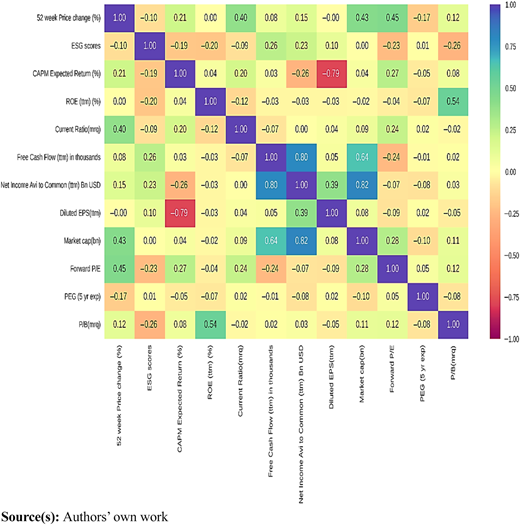
However, a notable and somewhat unexpected finding emerges concerning the correlation between diluted earnings per share (EPS) and CAPM-expected returns. Contrary to intuitive expectations, a negative correlation is observed, suggesting that as diluted EPS increases, the anticipated returns tend to decrease. This counterintuitive relationship prompts further inquiry, hinting that higher profitability on a per-share basis may paradoxically coincide with diminished expected returns. While these interpretations offer initial insights into the dynamics between the variables, it is essential to note that correlation does not inherently imply causation. Consequently, further in-depth analysis is warranted to elucidate the underlying reasons behind these observed patterns.
6.3 Results from K-means
6.3.1 Optimal number of clusters
The analysis employs the Elbow Method to ascertain the optimal number of clusters by evaluating distortion values across varying cluster numbers. Notably, the distortion, representing the average distance of points to their assigned centroid, exhibits a decreasing trend as the number of clusters increases. However, a distinct “elbow” point, signifying a significant reduction in distortion followed by a plateau, is not distinctly discernible in the plotted graph (Figure 5). Instead, the reduction in distortion appears to plateau gradually after approximately 3 or 4 clusters. This absence of a well-defined elbow complicates the determination of an optimal cluster count solely based on the Elbow Method.
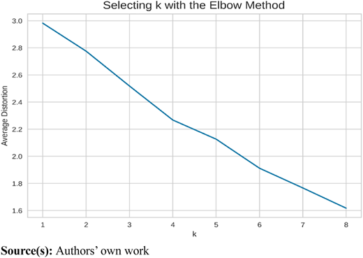
Furthermore, this gradual reduction in distortion is not uncommon in certain datasets, where the decline occurs smoothly rather than abruptly. The complexity of the dataset contributes to this subtlety; high variability in financial metrics and inherent noise in financial data lead to a more gradual decline in distortion. The dataset’s sectoral diversity and high dimensionality further complicate the formation of well-defined cluster boundaries. The silhouette scores exhibit variability across different iterations, as noted in the literature (Fränti and Sieranoja, 2019).
The average silhouette score across iterations is calculated to be 0.35, while the highest silhouette score observed is 0.42. Both metrics suggest a plausible range of clusters, with the highest silhouette score indicating optimal clustering with 3 clusters. Concurrently, the Elbow Method suggests a potential inflection point around 3 or 4 clusters, albeit without a distinct elbow formation. Notably, the Silhouette Score offers a more direct assessment of cluster separation, indicating that certain iterations resulted in well-separated clusters, evidenced by a score of 0.46. This convergence of findings from multiple evaluation methods underscores the robustness of the clustering analysis. Figure 6 illustrates the silhouette coefficient approach, revealing that four clusters display a slightly higher average silhouette coefficient value compared to three clusters. Consequently, we designate four clusters as the optimal choice and proceed to delineate the ensuing cluster profiles. Cluster 0 comprises a solitary security, notably an outlier, exemplified by an expected return of −27.6% and an exceptionally high diluted EPS of $52,660, attributed to Berkshire Hathaway.
This outlier warrants further scrutiny, advocating for a comprehensive financial analysis encompassing factors like financial statements, market dynamics, and industry trends to decipher the underlying reasons behind its outlier status. Cluster 1 encompasses 20 securities, boasting an average expected return of 12.42% and a notably high average return on equity of 259.6%, juxtaposed with a relatively low average net income of $10.22 billion. Remarkably akin to cluster 2, the primary discrepancy lies in the return on equity metric. Cluster 2 comprises 3 securities sharing close resemblance to cluster 1 across various metrics, albeit with a lower average return on equity (79.49%) and a higher average net income of $84.45 billion. Cluster 3 encompasses 26 securities characterized by relatively poor performance metrics compared to other clusters, featuring low average values across financial metrics, notably the sole cluster exhibiting a negative average 52-week price change.
Overall, clusters 1 and 2 are deemed safer investments, with cluster 2 comprising more exclusive securities, whereas clusters 0 and 3 denote riskier investments. Furthermore, a cross-tabulation between the “GICS Sector” and “K_means_segments” is conducted to discern the alignment between clusters generated by the K-means algorithm and sectors delineated by the Global Industry Classification Standard (GICS). This analysis, presented in Table 3, highlights the predominant sector within each cluster, offering valuable insights into clustering patterns. In the Healthcare sector, stocks such as DHR (with the highest expected return of 9.51%) and LLY (with the lowest return of 3.51%) both fall within Cluster 3, regardless of their differing risk-return profiles. This suggests that clustering in the healthcare sector is driven by sectoral alignment rather than variations in expected returns or beta values. In contrast, the IT sector demonstrates a stronger similarity between risk-return metrics and clustering. High-return, high-beta stocks like AMD are assigned to Cluster 1, while lower-return, more stable stocks like MSFT are placed in Cluster 3, indicating that IT clustering is more influenced by the magnitude of expected returns and risk factors than by sector alone.
Cross tabulation results
| K means segments | 0 | 1 | 2 | 3 |
|---|---|---|---|---|
| GICS Sector | ||||
| Healthcare | 0 | 1 | 0 | 9 |
| IT | 0 | 9 | 2 | 2 |
| Communication Services | 0 | 2 | 1 | 3 |
| Consumer Discretionary | 0 | 4 | 0 | 1 |
| Consumer Staples | 0 | 1 | 0 | 5 |
| Energy | 0 | 0 | 0 | 2 |
| Financials | 1 | 2 | 0 | 3 |
| Materials | 0 | 1 | 0 | 0 |
| Utilities | 0 | 0 | 0 | 1 |
Source(s): Authors’ own work
Similarly, in the Communication Services sector, stocks with higher expected returns, such as DIS and NFLX, are grouped in Cluster 2, while stocks with lower returns, such as VZ, are in Cluster 3. This pattern suggests that in this sector, clustering is more aligned with risk-return characteristics. In the Consumer Discretionary sector, high-return stocks like TSLA are assigned to Cluster 2, while lower-return stocks like MCD are in Cluster 3, indicating that clustering in this sector also depends on risk-return profiles rather than sector alignment. For Consumer Staples, the clustering pattern is like that seen in Information Technology and Consumer Discretionary, where KVUE (with the highest return of 21.08%) is placed in Cluster 1, while lower-return stocks like PG (4.68%) and WMT (4.84%) are in Cluster 3. This supports the idea that risk-return profiles significantly influence cluster assignments in this sector. In contrast, in the Energy sector, both CVX and XOM are assigned to Cluster 3 with relatively similar returns and betas, indicating that sectoral alignment is the primary driver of clustering in this case.
In the Financial sector, there is a wide spread across clusters, with high-return stocks like BAC placed in Cluster 1 and BRK, which has a negative return, assigned to Cluster 0. This highlights that risk-return profiles have a significant influence on clustering in the financial sector, as stocks with dramatically different returns and betas are assigned to different clusters. Finally, in the Materials and Utilities sectors, stocks such as LIN (9.46%) and NEE (4.65%) are grouped in Cluster 3, suggesting that in these sectors, clustering is more closely tied to sectoral alignment rather than distinct variations in risk or return.
Overall, we observe that the relationship between expected returns, beta values, and clustering varies by sector. In sectors like IT, Consumer Discretionary, and Financials, risk-return characteristics are the primary drivers of cluster formation, with stocks exhibiting similar risk-return profiles tending to fall within the same clusters. However, in sectors such as Healthcare, Energy, and Consumer Staples, sectoral alignment plays a more significant role in determining cluster assignment, with less emphasis on the magnitude of expected returns or beta values.
6.4 Agglomerative clustering results
The cophenetic correlation analysis results are presented below.
The highest cophenetic correlation obtained is 0.93, achieved with Euclidean average linkage. Despite the dendrograms in Figure 7 suggesting 4 as the optimal number of clusters, Euclidean average linkage clusters the majority of 44 stocks together out of the sample 50, resulting in limited variability that lacks utility.
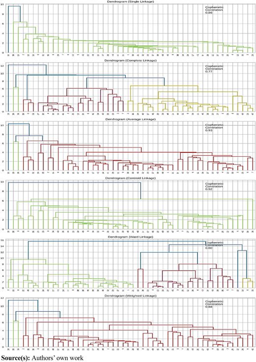
Consequently, we opt to conduct clustering using Ward linkage, which yields more distinct and separated clusters, as evidenced by the dendrogram in Figure 7. Once again, 4 appears to be the appropriate number of clusters from the dendrogram. Notably, the results closely resemble those obtained from the k-means algorithm, as presented in Tables 4 and 5. The agglomerative cluster profiles mirror the distributions and average financial metrics observed with k-means. To avoid redundancy, we refrain from reiterating them. Specifically, Cluster 0 bears strong resemblance to Cluster 1 from K-means, while Cluster 1 corresponds closely to Cluster 2 from K-means. Similarly, Cluster 2 mirrors Cluster 3 from K-means, and Cluster 3 aligns closely with Cluster 0 from k-means.
Cophenetic correlation results
| Distance metric | Linkage Method | Cophenetic Correlation |
|---|---|---|
| Euclidean | Single | 0.86 |
| Euclidean | Complete | 0.77 |
| Euclidean | Average | 0.93 |
| Euclidean | Weighted | 0.88 |
| Chebyshev | Single | 0.85 |
| Chebyshev | Complete | 0.81 |
| Chebyshev | Average | 0.89 |
| Chebyshev | Weighted | 0.86 |
| Mahalanobis | Single | 0.81 |
| Mahalanobis | Complete | 0.80 |
| Mahalanobis | Average | 0.84 |
| Mahalanobis | Weighted | 0.83 |
| Cityblock | Single | 0.85 |
| Cityblock | Complete | 0.67 |
| Cityblock | Average | 0.89 |
| Cityblock | Weighted | 0.80 |
Source(s): Authors’ own work
6.5 Agreement analysis between hierarchical clustering and K-means clustering
We assess the agreement between the clusters generated by Hierarchical Clustering (HC) from ward linkage and K-means Clustering using two metrics:
Adjusted Rand Index: 1.0000
The Adjusted Rand Index (ARI) quantifies the similarity between two clustering results. It adjusts for the chance grouping of elements, providing a value between −1 and 1. A maximum value of 1 indicates perfect agreement, meaning the two clustering outcomes are identical in terms of which data points are grouped together, while a score of 0 suggests that any similarity is purely random. The formula for ARI is as follows in Eq. (3).
where the Index is the raw count of similar cluster assignments between the two results, and E[Index] is the expected index under random clustering.
Here, the Adjusted Rand Index is 1.0000, indicating a perfect match between the clusters produced by agglomerative and K-means methods.
Cohen’s Kappa: 0.2208
Cohen’s Kappa measures the agreement between two clustering methods, while adjusting for the possibility of agreement occurring by chance. The formula for Cohen’s Kappa is in Eq. (4):
where is the observed agreement between the two methods, and is the expected agreement by chance.
A value close to 1 suggests high agreement, while a negative value, as observed (−0.2208), implies that the observed agreement is less than what would be expected by chance. While Cohen’s Kappa indicates lower agreement, the Adjusted Rand Index suggests a perfect match in clustering results. In our analysis, while ARI shows perfect similarity (because all the data points are paired in the same clusters), Cohen’s Kappa might see differences in how the clusters are distributed, leading to a lower Kappa score. Further exploration is warranted to understand the sources of discrepancy and agreement between agglomerative and K-means clustering. One potential reason for this discrepancy could be that clear clustering may not be occurring. Ideally, in real-time scenarios, it would be advisable to utilize multiple clustering algorithms provided by cloud providers to achieve the best results. Another reason could be that whereas ARI focuses on how data points are paired without considering cluster labels or sizes, Cohen’s Kappa considers the method behind the clustering and how balanced the clusters are as it measures agreement based on a contingency table and considers the overall frequency of matches and mismatches between the clusters.
6.6 Results from PCA
The plot aids in comprehending the trade-off between the number of principal components and the variance retained in the data (Figure 8).
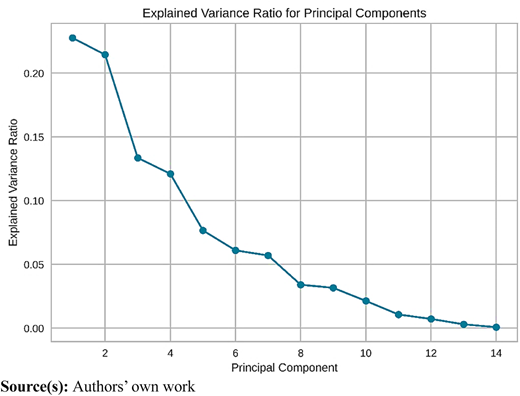
It reveals that the first two principal components collectively explain 44% of the variance in the dataset. Additionally, upon visual inspection, it is evident that both clustering methods produce similar outcomes (refer to Figure 9).
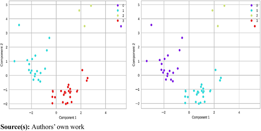
Left side represents K means and right side represents agglomerative clustering (Ward linkage)
Left side represents K means and right side represents agglomerative clustering (Ward linkage)
7. Conclusion
In this study, we conduct a thorough fundamental analysis of securities, leveraging a range of risk and return metrics. The CAPM serves as the cornerstone for estimating Betas and expected returns, forming the basis for clustering stocks. Our comparison of the performance of clustering models reveals striking similarities, offering insights into the trade-offs associated with different cluster numbers. The applications of such analysis are manifold. The comprehensive yet straightforward approach we employ can be readily extended to further explorations in the portfolio management domain. For instance, a portfolio management firm could utilize similar clustering techniques to propose diverse sets of stocks tailored to individual clients' risk preferences (Bariviera et al., 2023). Moreover, employing clustering to identify varying levels of risk appetite among customers enables the customization of security recommendations, enhancing client satisfaction and portfolio performance (Mariani and Mancini, 2024).
A logical progression from our current study could involve employing multi-factor models as the foundation for clustering, thereby integrating additional dimensions of risk and return. Alternatively, exploring alternative unsupervised clustering methods such as Fuzzy C means could be beneficial, particularly in scenarios where data points may exhibit membership in multiple clusters simultaneously. However, it’s important to acknowledge the limitations inherent in our study. The CAPM, while widely used, rests on assumptions such as market efficiency and homogeneous investor expectations and risk preferences (Mullins, 1982), which may not hold true in real-world settings. Consequently, deviations from these assumptions could impact the accuracy of expected returns predicted by the model. Furthermore, while our clusters reveal statistical patterns, ascribing economic or financial rationale to each cluster may introduce subjectivity and complexity into the interpretation.
Conflict of interest statement: There is no conflict of Interest
Data availability: Data is collected and available from the Yahoo Finance website.
