


Deforestation from timber harvests and farmland conversions have led to 565 GtCO2 (billion tons of carbon dioxide) being emitted into the atmosphere. Taking into account natural regeneration on forestland, Houghton (2003, 2008) and Houghton et al. (2012) estimate that deforestation has caused a net loss of 484 GtCO2 since 1900 which is about one third of all manmade emissions. However, these estimates do not take into account the substantial investment into fire management, plantations, and replanting since 1950, as well as the effect of carbon fertilization on a younger forest. We compare the outcome of a deforestation scenario with subsequent forest management with what would have happened if the natural forest in 1900 had not been harvested thereafter. Deforestation plus forest management suggests current forests actually hold about 94 GtCO2 more today than they did in 1900. However, natural forests would have held an additional 186 GtCO2. Human activities on forestland have therefore caused about 92 GtCO2 of net emissions since 1900. The effect of manmade land use and land use change is relatively small compared to the 1294 GtCO2 from industrial emissions over the same time period (Marland et al., 2008).
1 Introduction
This paper questions the long-standing assertion that manmade land use and land use change has caused almost one third of total anthropogenic emissions of carbon dioxide (CO2) (IPCC, 2013).1 The paper starts with the landmark estimate of 565 GtCO2 historic emissions from deforestation made by Houghton (2003, 2008) and Houghton et al. (2012). This gross emission was caused by 1 billion hectares of old growth forest being harvested (FAO, 2012) and 700 million ha of forestland being converted to farmland (Houghton, 2003, 2008; and Houghton et al., 2012) since 1900. Assuming that cut over forests regenerate naturally, Houghton (2003, 2008) and Houghton et al. (2012) estimate that the net effect of deforestation was 484 GtCO2 since 1900. This paper questions this net estimate because it does not include the substantial investment in forests that has happened since 1950. If investments in growing and protecting forests are included in land use and land use change, the net effect of manmade land use and land use change on carbon emissions is much smaller.
Most of the world’s standing forest in 1900 had never been cut. The major exception was in Europe which had been practicing renewable forestry2 since the middle of the 19th century. Except in Europe, the global forest was composed largely of mature stands. Except in Europe, forestry throughout the first half of the 20thcentury followed the assumption of Houghton and did not replant or manage forests at all. As assumed by Houghton, the only regeneration in these non-European forests was natural. However, beginning in the 1950’s, a vast amount of global forest came under some level of manmade forest management. Both the private sector and governments invested billions of dollars in planting, fire control and other forest management activities aimed at increasing the growing stock, growth rate, and/or value of forests. These management activities include a wide range of site-specific activities, including changing species type, improving genetics through selection, altering planting intensity, controlling competition, thinning, fertilizing,3 improving drainage, and irrigating. Increasing the intensity of growth on more productive forestland focuses harvesting on fertile forestland, so that most global forestland today remains in a natural and unharvested state.
Forestry moved from being a nonrenewable mining activity (depleting an existing forest stock) to a renewable activity (maintaining a renewable forest stock) over the twentieth century. With the renewable stock, the forestry investments offset harvests, thus maintaining the underlying stock. By converting the slow growing mature forest into a younger faster growing forest, the investments have also taken advantage of the increased growth rate of trees from carbon fertilization. The younger forest has made global forests a more active sink for carbon than the original mature forest. The combination of these market investments and carbon fertilization have helped forests more than regain the original carbon lost from deforestation. This paper compares how much carbon an untouched natural forest would have stored since 1900 with how much carbon forests actually lost and then regained from both deforestation and subsequent forest investment.
This paper answers this question with an economic-ecological model of global forests, the Global Timber Model (Sohngen et al., 1999). The Global Timber Model (GTM) is an optimal control model of the global timber market (Sohngen et al., 1999). The model provides a dynamic simulation of how forests and forest management changes over time because of both ecological and market forces. The model maximizes the net present value of timber harvests over time subject to the constraint of an initial stock of available timber and assumptions about the supply of timber over time. The model has previously been implemented to start with current stocks and look forward (e.g., Sohngen et al., 1999; Sohngen et al., 2001; Daigneault et al., 2012; Favero and Mendelsohn, 2014; Tian et al., 2016).
For this study, however, we use the model to look backwards and study the historical period, starting with mature timber in 1900 and observations about the supply and demand for timber from 1900 to 2010. The model relies on an ecological model for local growth, biomes, and biomass in 250 forests around the world given climate and CO2 concentrations. The economic features of the GTM model are also able to reproduce both the nonrenewable and renewable phase of forestry. The GTM reproduces historic timber harvest rates and management back to 1900. The GTM also simulates historic harvest, planting, and management intensity in each forest around the world. The “Historical Market Scenario” simulates historic harvests and forest investments and explains what actually has happened to forests.
We then contrast this Historical Market Scenario with the “Natural Forest Scenario”. The Natural Forest Scenario is a hypothetical case that assumes that humans left the 1900 forest alone and nature took its course through time. No stands are harvested or converted and only ageing, natural disturbances (largely fire), and natural regeneration of lost forests occurs. In both scenarios, we assume that the forest was exposed to the observed historic concentrations of CO2 in the atmosphere.4 We measure the net effect of manmade land use and land use change as the difference in forest carbon held by the Natural Forest Scenario versus the Historical Market Scenario.
The results of the Natural Forest Scenario suggest that the carbon fertilization effect on the untouched natural forest would have increased the stock of forest biomass by 186 GtCO2 between 1900 and 2010. If forests had been left alone, they would have acted as a sink for atmospheric CO2. The modeled effect of deforestation, investments in managed forests, and carbon fertilization in the historical market scenario reveals that forest biomass increased by 94 GtCO2 between 1900 and 2010. Despite the extensive deforestation, the combination of forest investment and carbon fertilization has meant that the actual historic forest has also been a small net sink of atmospheric CO2. However, the Natural Forest Scenario would have been a slightly larger sink, storing 92 GtCO2 more carbon from 1900 to 2010. This additional 92 GtCO2 is the net emission from manmade land use and land use change. This is substantially smaller than the net emission estimated by Houghton (2008) and Houghton et al. (2012) of 484 GtCO2 assuming no forest investments at all. Section 2 describes the economic theory explaining why forestry was at first a nonrenewable resource industry but subsequently became a renewable industry (Berck, 1979). Section 3 describes the details of the ecological- economic Global Timber Model (GTM) and the details of the two scenarios. Section 4 describes the results of each scenario. The paper concludes with some general observations and reservations about the experiment. Even though the paper argues that deforestation and forestland change may have contributed only a small share of historic anthropogenic emissions, the conclusion notes that forestry is potentially a very important source of future carbon mitigation.
2 Theory
Markets had three impacts on land use and land use change. There was a conversion of substantial forestland into farmland, there was an extensive harvest of most of the world’s accessible mature forest, and there was a subsequent investment to renew the forest. The rapid growth in population in the 20th century substantially increased the demand for food and caused a lot of forestland to be converted to farmland. We model this land-use change exogenously over time to reflect actual decadal conversion rates. We assume that land conversion to farmland happened on clear-cut forestland so that it did not contribute to the loss of valuable forest stock.
We use GTM to simulate the historic impact of markets on global forests. GTM provides a theoretical and empirical model that replicates the behavior of the timber market. The theoretical model is an optimal control model which maximizes the present value of timber over time. Because the world’s forests were originally composed of an extensive mature stock of timber in 1900, there was more standing timber than the market could immediately use. In fact, it took the market about 90 years to harvest the bulk of the accessible old growth. Most of the remaining old growth forest today lies in either protected areas or inaccessible regions. The original abundant forest stock caused timber prices to initially be quite low. At these low prices, it was not profitable to replant timber. There was virtually no replanting before the 1950’s (except in Europe) and limited replanting for the first few decades thereafter. As long as this excess stock existed, forestry was a nonrenewable industry. The forest industry’s goal was to mine (deplete) the stock of standing mature timber. Maximizing the value of this standing timber requires the price of timber to rise nearly at the interest rate (Hotelling, 1931). The historic price of timber did in fact rise at nearly the interest rate.
The nonrenewable resource model also predicts that the market should completely deplete the entire accessible resource. The future substitute for this nonrenewable forest stock was a brand new renewable forest. The date at which the nonrenewable resource, the accessible mature forest,5 should be completely harvested depended upon the price of timber at which this renewable forest could be built to replace it. The price of the nonrenewable forest just as it is finally depleted should be equal to this renewable resource price.
The renewable forest, in turn, must be planted in advance so that it is ready the date the nonrenewable forest depletes. The renewable forest is limited to the land that is still in forests. This planting must begin a full rotation before the renewable forest is to begin. There is consequently a period during which the renewable and nonrenewable phases overlap. The market is still depending on the mature standing timber for harvests but there is also a planting and ongoing management of the renewable forest. From the perspective of the forest industry, the renewable phase was motivated by a timber gap- a forecast that timber demand would eventually exceed the available supply of mature timber left.
Another dynamic factor running through the model is the effect of climate change and carbon fertilization on forests. Both factors depend on the atmospheric concentration of CO2 which is growing over time because of the 1294 GtCO2 emitted by industrial sources (Marland et al., 2008). In this paper, the concentrations of CO2 in the atmosphere are assumed to be exogenous. We simply use the observed levels. However, because the model is reproducing historic forest choices, the observed CO2 in the atmosphere is exactly what it should be given how forests were actually managed. How forests responded to the changing climate and CO2 concentrations is captured by the ecological model, MC2, which simulates how higher levels of CO2 and climate change affect net primary productivity, NPP (Kim et al., 2017). We assume changes in NPP led to proportional changes in instantaneous growth.
In the natural forest scenario, we assume that the natural forest also grows faster because of the elevated atmospheric CO2 concentrations over time from industrial emissions (Norby et al., 2005). This slightly overestimates the CO2 concentrations in the natural forest scenario because there was slightly more carbon in the forest in this scenario. This means that we slightly overestimate how much the natural forest grew over this period and slightly overestimate the difference in carbon sequestration between the two scenarios.
We assume throughout that the volume/ha, V , is an S shaped function of age, a, and can be enhanced by investments into forest management, m:
where d is the maximum volume per hectare in each forest type and b is a growth parameter. The parameters, a and d, vary across forests and site quality. Volume can be increased above natural rates, which we normalize to 1, with expenditures on management. In the nonrenewable phase, the trees are all natural so that f (m) = 1. The harvested trees are assumed to be mature (old) during this initial phase, so that the forest according to (1) has high volumes/ha and is growing quite slowly.
The quantity of timber supplied, QS, is equal to the volume of timber/ha, V , times the number of hectares cut, x(t). The quantity supplied is approximately:
The nonrenewable phase seeks to maximize the present value of future harvests given that there is a finite stock of existing standing timberland, X0. The timber quantity demanded, QD(t), depends on price, PNR(t) at each moment t.
The gross benefit of timber consumption at each moment is the consumer surplus or integral under the demand function up to the timber price. The net value of the timber each moment is the gross value minus harvest costs per acre, HC. The net present value discounts these estimates to the present time using a constant discount rate, r. The net present value at each moment in time is therefore:
The overall problem during the nonrenewable phase is to find a harvest path that maximizes the overall value of harvesting the aggregate area of mature stock, X0:
The solution to this problem equilibrates the present value of the net price of timber (price minus cost) throughout the nonrenewable phase:
Rearranging terms, the timber price should rise over time at the following rate:
Prices rise at a rate slightly less than the interest rate. The terminal condition of the nonrenewable model, in year TT, is that the accessible stock of mature timber is exhausted:
If there is no substitute supply, this would mark the end of timber production. However, it is possible to establish a renewable timber supply by planting trees in advance for future harvest. Forest area is then replanted once harvested. If the market plants enough trees in advance for each future year of harvest, the market can sustain a sufficient flow of timber to meet demand indefinitely. Renewable forestry was first implemented in Germany in the mid-19th century to meet domestic needs. However, the global program to create a renewable forest did not begin until the 1950’s. This was a full rotation in advance of when the last of the world’s accessible mature timber was expected to be depleted (in the 1990’s).
The renewable price, PR, equates the supply of timber to the demand for timber. The renewable price is the ceiling price for PNR. Mature timber (from the nonrenewable phase) cannot be sold for more than PR. The optimal solution for the nonrenewable phase is that the nonrenewable price just equals the renewable price when the transition happens between them: PNR(TT) = PR. The nonrenewable price path just reaches the renewable price as the last of the stock of accessible mature timber is harvested.
The renewable resource price equilibrates the demand for timber, QD, Equation (3), with the renewable supply of timber, QS. The renewable supply each year is the product of the volume/ha of forest, V (T, m), where T is the age of the tree when harvested, times the forestland, x(t), available to harvest each year:
If the forest has x(t) hectares of trees of each age, the total size of the renewable forest, XR, must be:
There must be an age class for each future year of harvest. The supply function for additional forestland for the renewable forest, XR, comes from farmland, F (WR), and inaccessible natural forest, N (WN ):
where WF is the price of farmland and WN is the price of inaccessible natural forest. If the price of farmland exogenously increases (decreases), this implies that forestland will be converted to (from) farmland. Inaccessible natural forest tends to be mature timber that was too far from market to be harvested during the nonrenewable phase. The higher price of timber during the renewable phase makes some of these forestlands profitable to harvest. An equilibrium amount of forestland is reached when the price (marginal value) of farmland, WF , is equated with the price of inaccessible natural forestland, WN , is equated with the price of renewable forestland, WR.
The value of land in a renewable forest is the present value of income/ha, WR, that a landowner can earn (Faustmann, 1849):
A derivation of the Faustmann formula is provided in the Appendix. The expression in brackets is the net income from a single rotation. The net income in each rotation is the present value of the net revenue from selling the fully-grown trees at age T minus harvest cost, HC, the cost of planting, C0, and the cost of management, Cm(m). Earnings depend on the price of timber, PR, and the quantity of timber V (m, T ). The present value depends upon the interest rate, r, and the rotation length, T . The present value of an infinite series of forest rotations of length T requires the numerator to be divided by (1 − e−rT ).
Planting new rotations increases productivity relative to a natural forest by shortening the time for a rotation to begin and by assuring that the new stand is fully stocked. Management also increases productivity (Equation 1). Both planting and management cause the new managed forest to be more productive and hold more carbon than equivalent aged natural forests.
Differentiating (13) with respect to m and setting the result to zero yields the ideal intensity m∗ that maximizes π:
The present value of the future increase in marginal revenue from more management equals the marginal cost of m.
Differentiating (13) with respect to T yields:
which simplifies to:
The left-hand side of equation 15 represents the marginal benefit of holding timber another year. The first term is the benefit from the growth of the forest for another year. The second term is the benefit (loss) if the price of the standing timber increases (falls). For example, if the demand for timber grows (falls)over time, this will put upward (downward) pressure on the timber price and lengthen (shorten) rotations. The right-hand side of equation 15 reflects the marginal cost of holding the trees another year. The first term is the marginal cost of postponing harvest-the lost interest on the net sale value of the standing trees. The second term is the marginal cost associated with the income from delaying all future harvests. The solution to (14) determines the length of each rotation T . This in turn determines the volume of timber per hectare V (m, T ).
The supply function for land is not static in this model and depends upon the demand for agricultural land. The historic demand for farmland, F , grows in this model over time as population and income exploded in the twentieth century. R(X, F ) rises over time. Consequently, some of the original forestland, X0, is converted to farmland over time.
The renewable component of the model is quite consistent with a competitive market. If forestland owners are trying to maximize profits given market prices, they will face the same marginal conditions as stated in the equations above. Competitive forces will pressure supply to equal demand and for the marginal value of all three land uses to be equal.
As shown by Hotelling (1931), a competitive market efficiently extracts nonrenewable resources. Owners of the initial forest will choose when to harvest to make the most profits. Competition will encourage them to choose a strategy that leads to the same marginal profit across all time periods. If owners cannot affect price, competition leads to (7). Maximizing profit also encourages all forest owners of the initial mature timber to sell all their timber before prices reach the renewable price.
The natural scenario does not depend on the theoretical model at all because the natural scenario assumes that there is no human-driven harvesting or conversion of land. The natural scenario is subject only to the forces of nature. Trees are expected to age given their volume age function (Equation 1). Natural disturbances, natural regeneration, and the effect of climate change and carbon fertilization are all obtained from the dynamic vegetation model MC2 (Kim et al., 2017).
3 Global Timber Model (GTM)
The GTM is built around the theoretical model of how the market for timber works
from around the world. Within each forest, the model tracks the quantity of hectares by age class. The exogenous loss of forestland each past decade has been included in the model based on Houghton (2008) and Houghton et al. (2012). Each of the 250 forest types has its own growth function parameters (Equation 1). The dynamic vegetation model, MC2 (Kim et al., 2017), simulates NPP given the historic climate, soils, and CO2 at each location and time period. Carbon fertilization has been a major factor increasing forest growth. Doubling carbon dioxide concentrations increases forest NPP by 65% (Smith et al., 2009; Cramer et al., 2001; Norby et al., 2005; Scholze et al., 2006; Boisvenue and Running, 2006). The desired management intensity of newly planted stands is determined endogenously by balancing marginal costs and marginal benefits (Equation 14). The desired rotation length (harvest age) within each forest is determined endogenously by balancing the marginal gain of waiting versus harvesting (Equation 15).
The model maximizes the net present value of timber revenues subject to the initial stock of mature forestland, the instantaneous rate at which trees grow, and the endogenous price of timber. In this analysis, the price of carbon is set to zero, implying there is no carbon mitigation program causing the market to intentionally sequester carbon in forests. To the extent that carbon is sequestered in forests, it is simply a byproduct of growing timber for markets (or natural forest growth). The global demand for timber, Equation (3), is estimated to have the following specific form:
where b is the growth rate of timber demand. Between 1900 and 2010, average global income per capita rose from $1263 to $6038 (Maddisson, 2010). Over this same period, global population rose from 1.6 billion to 6.1 billion (Maddisson, 2010). Both of these forces led to a steady increase in global demand for timber over time. This has continued with the renewable forest which has increased the price of timber over time (although at a slower rate than during the nonrenewable phase).
The historic increase in income and population also led to a surge in the demand for agricultural products. Because the demand for food is rising faster than the increases in farm productivity, the global demand for farmland has been increasing. Forestland has consequently been converted to farmland. We utilize Houghton (2008) to construct forest area estimates for each continent for 1900. There is no data on precise age class distributions of global forests in 1900, but because most of this forest was never harvested, we assume these forests are mature, except in Western Europe where many forests were already being managed renewably by 1900. In Western Europe, we assume that forests in 1900 had even amounts of hectares in each age class up to the desired rotation length in this region. The model calculates that 700 million ha of forestland have been converted to farmland since 1900 and that 36 million ha of temperate farmland has returned to forest since 1900. Table 1 shows the change in aggregate forestland by continent.
Total Forest Area (in Millions of Hectares) over historical period (1900–2010)
| Intensive Plantations | Moderately Intensive Management | Primary forest (low intensity use) | Total | |
| North America | ||||
| 1910 | 0.0 | 0.3 | 642.9 | 643.2 |
| 1960 | 12.1 | 44.8 | 601.4 | 658.3 |
| 2010 | 27.3 | 108.4 | 561.9 | 697.6 |
| Europe | ||||
| 1910 | 0.0 | 0.6 | 1114.6 | 1115.1 |
| 1960 | 22.8 | 32.9 | 970.1 | 1025.8 |
| 2010 | 44.8 | 120.3 | 902.6 | 1067.6 |
| South & Central America | ||||
| 1910 | 0.0 | 2.1 | 1204.3 | 1206.4 |
| 1960 | 5.6 | 37.5 | 1136.8 | 1179.9 |
| 2010 | 13.1 | 40.3 | 957.1 | 1010.5 |
| Asia | ||||
| 1910 | 0.4 | 0.0 | 703.6 | 704.0 |
| 1960 | 11.7 | 0.0 | 624.8 | 636.6 |
| 2010 | 47.2 | 40.1 | 490.6 | 577.9 |
| Rest of World | ||||
| 1910 | 0.0 | 0.0 | 1254.7 | 1254.7 |
| 1960 | 2.6 | 0.0 | 1134.6 | 1137.3 |
| 2010 | 7.8 | 1.8 | 905.5 | 915.0 |
| World | ||||
| 1910 | 0.4 | 3.0 | 4920.0 | 4923.4 |
| 1960 | 54.8 | 115.3 | 4467.8 | 4637.9 |
| 2010 | 140.2 | 310.9 | 3817.6 | 4268.7 |
Note: Europe includes Russia.
There are large differences in ecological conditions in different parts of the world, from fast-growing regions with high NPP in the tropics and subtropics, to slower growing regions in the boreal zone. While expanding the model to multiple ecosystem types complicates solving the model, it does not alter the theoretical model above, which can be generalized to many supply regions.
The parameters for the volume-age function are estimated from data on wood volumes and age classes, such as the Forest Inventory and Analysis (US Forest Service, 2016). Because data on yield functions for 1900 are not available, we make several additional assumptions. Forest yields have generally risen over the century. This is partly due to forest fire suppression, but it is also due to nitrogen deposition, carbon fertilization, and climate change (see e.g., Smith et al., 2009; Cramer et al., 2001; Scholze et al., 2006; Boisvenue and Running, 2006). The model assumes that all of these factors have increased the productivity of forests on average by 0.08%/yr from 1900–1950, rising to 0.4%/yr by2010. These estimates are consistent with the estimates of Scholze et al. (2006), who suggest that in the absence of deforestation, forests have sequestered roughly 3.67 GtCO2 per year since the 1950s.
The largest contributor to increased growth was from carbon fertilization. CO2 concentrations increased from 290 to 389 ppm (32%) from 1900 to 2010. According to several ecological studies, doubling CO2 increases forest NPP by 65% (Norby et al., 2005). The 32% increase in CO2 over this period therefore increased NPP (annual growth) in forests by about 20% (Norby et al., 2005). Warmer temperatures and greater precipitation likely also increased NPP over this time period by about 3% (Gerber et al., 2004; del Grosso et al., 2008). Note that this historic beneficial effect of warming on forest ecosystems, may not continue into the future as temperatures continue to rise (Scholze et al., 2006; Friedlingstein et al., 2006; Frank et al., 2010).
While the historic increase in NPP has increased the amount of carbon being captured by forests, other factors may cause more carbon emissions. Higher temperatures may increase soil respiration and increase forest fires (Friedlingstein et al., 2006; Gonzalez et al., 2010; Friedlingstein and Prentice, 2010). In practice, forest fires have been suppressed (managed). The actual land area burned in regions like the United States is about 85% less than the natural rate simulated by ecological models. Fire management has consequently led to higher forest volumes and more carbon being stored in forests than ecological models would otherwise suggest.
In 1900, harvested timberland was naturally regenerated each year (gt) except in Western Europe. The model solves for the time when planting became profitable (the beginning of planting for the renewable forest) starting in 1950 in the United States and expanded to other regions in subsequent decades. Natural regeneration is associated with low intensity management (just fire control), planted forestland is associated with medium intensity (modest fertilization and insect control), and plantations are associated with high intensity fertilization and pest control. Increasing intensity leads to denser plantations which grow faster. The speed and magnitude of the volume age function increases, leading to more carbon storage at every moment in time.
The model assumes a perfectly competitive forest market with well-developed private property rights. Around 80% of the world’s forests, however, are government owned (UN FAO, 2010). In many developing countries, private individuals often live within forests. In these public forests, individuals do not necessarily maximize the present value of either consumer surplus or profits. Public lands that are leased to companies to harvest are included in the forest base. The model treats public forestland that is not leased for harvest as “inaccessible forest” that is not managed or harvested. The model assumes that there is a cost to harvest this inaccessible forest that keeps most of this forest from supplying timber. However, some of these forests are “illegally” harvested, harvested without explicit permission from the government. We assume that these illegal harvests are naturally regenerated.
4 Results
The historical market scenario begins with the assumption that timber demand increased steadily over the twentieth century as population and income increased. Timber supply also increased. Figure 1 traces the change in harvests in each major forest region since 1910. Both recent data and model output suggest that timber harvesting has increased over the entire twentieth century in every region. In the early twentieth century, North America and Europe (including the European part of Russia) supplied most of the global industrial timber. In the second half of the 20th century, global output was split with the rest of the world. Timber from North America and Europe fell to about 25% each, while the share of total output from Latin America and Asia increased to 25% and 15% respectively. These results, while not identical, mirror other historical data from 1960 to the present (FAO FAOSTATS, 2014). Timber harvests account for a great deal of the deforestation throughout the twentieth century. Overall, more than 1 billion ha of accessible mature forest stands were deforested over this period (Houghton, 2008).
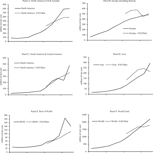
Timber output simulated by region for historical market scenario from 1900 to 2010, plus timber output for comparable regions from the UN Food and Agricultural Organization for 1960–2010.
Timber output simulated by region for historical market scenario from 1900 to 2010, plus timber output for comparable regions from the UN Food and Agricultural Organization for 1960–2010.
Another major impact of land use on forest carbon is from the conversion of forestland to farmland (see Table 1). Over the twentieth century, 700 million ha of mature forestland were converted to farmland (Houghton, 2008; Houghton et al. (2012)). About 540 million ha of these forests were converted to cropland (Ramankutty and Foley, 1999). This increase in cropland was concentrated in the tropics with 158 million ha in Latin America, 55 million ha in sub-Saharan Africa, 250 million ha in tropical Asia, and 37 million hectares in the Pacific (Ramankutty and Foley, 1999). The remaining loss of forestland went to grazing land. In 1900, there were 4.9 billion ha of forest. With land use conversions, there are 4.2 billion ha of forest today.
The price path of timber projected by the model rises almost at the rate of interest. Figure 2 shows that actual historic United States log prices from 1900–2010 are very close to these model price simulations. The historical growth rate of timber prices for the United States is around 2.3% per year (Haynes, 2008) from 1900–1990. The model results suggest that real (inflation adjusted) historical timber prices increased at 1.9% per year from 1900–1990. The model may have underestimated how fast prices increased because it overestimated harvest costs in the early half of the century due to the absence of environmental regulations during this period.
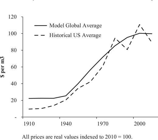
Historic United States log prices for 1900-2010 (Haynes 2008) and endogenous model prices in the historical market scenario.
Historic United States log prices for 1900-2010 (Haynes 2008) and endogenous model prices in the historical market scenario.
A third effect of land use on carbon is the increase in forestry investments that began around the middle of the last century. Before 1950, some harvested stands in the United States were converted to farmland but most forestlands were left to regenerate naturally. After 1950, however, more of the harvested stands were replanted in the United States in anticipation of a timber shortage that was predicted by the 1990’s as the United States ran out of mature timber (Kauppi et al., 2006). This is consistent with what the model finds for the United States. A large share of the mature timber harvested in tropical countries was converted to farmland with the remainder being abandoned for natural regeneration. It was not until the 1980’s that substantial replanting began in tropical forests around the world. This again is one rotation before the transition to the renewable forest as suggested by the model.
In the 1990’s, mature timber was no longer the primary source of timber in global markets. Timber, by this point, was largely coming from secondary forests that had either regrown naturally or had been replanted. By 2010, there were 290 million ha of moderately intensively managed forestland and 142 million ha of intensively managed plantations. These forests are growing at a faster rate than naturally regenerated forests and they all have more carbon per ha than naturally regenerated forests. Table 2 calculates the emissions (from harvest) and subsequent sequestration that has happened on these managed forests. For the historical market scenario, the model simulates that the overall effect of deforestation, forest investment, and carbon fertilization has added the equivalent of 94 GtCO2 to forests from 1900 to 2010. Forests hold slightly more carbon now than they did in 1900. Much of this increase occurred in North America and Europe. This result is supported by carbon balance models that trace the stocks of carbon in the ocean, atmosphere and land. The carbon models also calculate that there is slightly more carbon in the land today than in 1900 (IPCC, 2013a).
Cumulative Change in Forest Stocks (GtCO2) from 1900–2010
| Natural Forest Scenario | Historical Market Scenario | ||||||
| Managed | Un-Managed | Total | Managed | Un-Managed | Total | ||
| GtCO2 | |||||||
| North America | Loss | −10.4 | −6.2 | −16.6 | −24.5 | −29.6 | −54.1 |
| Gain | 10.6 | 0.9 | 11.4 | 71.0 | 54.8 | 125.8 | |
| Net | 0.2 | −5.4 | −5.2 | 46.6 | 25.1 | 71.7 | |
| Europe | Loss | −49.9 | −20.4 | −70.4 | −25.5 | −47.4 | −72.9 |
| Gain | 50.3 | 69.1 | 119.4 | 34.8 | 93.5 | 128.4 | |
| Net | 0.3 | 48.7 | 49.0 | 9.4 | 46.1 | 55.5 | |
| South and Central America | Loss | −0.5 | −73.9 | −74.4 | −72.3 | −203.7 | −276.0 |
| Gain | 1.9 | 151.3 | 153.2 | 84.5 | 194.3 | 278.8 | |
| Net | 1.4 | 77.4 | 78.8 | 12.2 | −9.4 | 2.8 | |
| Asia | Loss | −30.8 | −26.9 | −57.7 | −48.8 | −86.1 | −135.0 |
| Gain | 31.2 | 89.3 | 120.4 | 67.9 | 79.3 | 147.2 | |
| Net | 0.3 | 62.4 | 62.7 | 19.1 | −6.8 | 12.3 | |
| ROW | Loss | 21.9 | −24.9 | −3.0 | −73.8 | −126.0 | −199.8 |
| Gain | −22.2 | 25.4 | 3.2 | 71.2 | 80.2 | 151.4 | |
| Net | −0.3 | 0.5 | 0.2 | −2.6 | −45.7 | −48.4 | |
| World | Loss | −69.8 | −152.4 | −222.2 | −244.8 | −492.9 | −737.7 |
| Gain | 71.8 | 335.9 | 407.7 | 329.4 | 502.1 | 831.5 | |
| Net | 2.0 | 183.5 | 185.5 | 84.6 | 9.3 | 93.8 | |
Notes: Europe includes Russia; Gigaton (GtCO2) is a billion metric tons of carbon dioxide. Above and below ground biomass, soil carbon, and material on the forest floor including slash and other debris are all included. Model assumes that 25% of aboveground biomass is emitted immediately with forest fires in the natural forest scenario.
Table 2 also presents the natural forest scenario, where we assume no deforestation, no harvesting, and no fire management, and illustrates that a natural system also would have accrued more carbon over the period 1900 to 2010. This accumulation was largely in response to carbon fertilization which made all forests grow faster. Without human intervention, the natural scenario suggests that the stock of carbon in trees would have grown by the equivalent of 186 GtCO2 by 2010. Comparing this estimate to our simulated increase in forest carbon under the historical market scenario, the natural forest would have grown an additional 92 GtCO2 by 2010. The difference (92 GtCO2) between the outcome in the natural forest and the actual forest is the net emissions from land use and land use change.
5 Conclusios
This paper examines the role of forests in the global carbon cycle. We utilize the gross deforestation estimates since 1900 by Houghton (2008) and Houghton et al. (2012). However, we recalculate the net estimates made by Houghton (2008) and Houghton et al. (2012). The Houghton net estimate assumes that harvested forests would regrow naturally after being clearcut. In practice, however, a substantial area of forest has been planted and managed. The net effect of land use and land use change is much smaller than what Houghton first estimated.
We recreate historic harvests and investments that have been made in global forests using a forest model, GTM. The model explains why markets at first treated forests as a nonrenewable resource but then shifted to managing forests as a renewable resource. The model tracks historic data closely. This model explains the observation that modern forests contain almost the same stock of carbon as the 1900 forest did even though much forestland has been lost to farmland. If forests had regenerated naturally, the remaining forestland would not have been able to recover all this lost carbon. The paper contrasts this historic actual outcome with a hypothetical “Natural Forest” scenario where the 1900 forest is not deforested or managed. This hypothetical case reveals that an untouched natural forest would have sequestered even more carbon than the actual forest has. The difference is the net effect of land use and land use change. The results suggest that land use and land use change caused a net emission of 92 GtCO2. This net estimate is considerably smaller than the net estimate by Houghton (2008) and Houghton et al. (2012) of 484 GtCO2. Given that industrial sources from 1900–2010 emitted 1294 GtCO2 (Marland et al., 2008), the net effect of land use and land use change on cumulative manmade CO2 emissions is 7%.
One must be careful not to use past trends in land use to forecast the future. The last century was a period of great upheaval as the world’s mature forests were converted to farmland, young secondary forests, and managed forests. Those vast changes will not continue into the future. Very little mature forest will be harvested in the future as the world now largely depends on secondary and managed forests for timber. The large increase in 20th century farmland is not projected to continue into the future (Hertel et al., 2009). Because carbon fertilization is a function of the log of CO2 concentrations, the carbon fertilization effect will increase at a decreasing rate.
The analysis does not present formal estimates of the uncertainty surrounding the results but the reader should be aware that there is uncertainty in measuring carbon over time. Even small errors in measuring the very large stocks of carbon in forest biomass, debris, and soils lead to large errors in predicting changes in those stocks. Records of exactly how much timber was harvested in the first half of the twentieth century for the entire world are incomplete. The total volume per hectare of global forests in 1900 was also not measured carefully. The carbon fertilization effect on tree growth in every forest around the world is uncertain. The natural disturbance rate from forces such as fire in the absence of fire control is uncertain. However, it is highly likely that the sizable investment of forestry into replanting and management had a sizeable effect on the carbon in today’s forests. The commonly stated summary of the literature (e.g., IPCC, 2013a) that one third of anthropogenic emission comes from land use and land use change does not take this investment into account. It is highly likely that the net effect of land use and land use change is much smaller (approximately 7%).
It is important to emphasize that the results of this study concern just historical emissions of CO2. Forests may have a very large role in future efforts to mitigate CO2. The world’s forests can readily sequester more carbon than they do now if governments provide an incentive for forest owners to store carbon. As the incentive grows, more and more carbon can be set aside in forests. For example, a CO2 price of $17/ton would lead to an additional 147 GtCO2 and a price of $50/ton would lead to an additional 367 GtCO2 stored in forests (Sohngen and Mendelsohn, 2003). If carbon prices reach $400/ton, 1285 GtCO2 could be stored in global forests (Sathaye et al., 2007). Forests can also provide bioenergy which when combined with carbon capture and storage, can potentially remove CO2 from the atmosphere (Favero and Mendelsohn, 2014, 2017). Even if the role of land use and land use change in historic carbon emissions has been relatively small, forests can still be an important part of the solution to curbing global warming.
Note
Correspondence author: Brent Sohngen, sohngen.1@osu.edu
Calculated from Figure 6.8 in IPCC (2013). This paper focuses on carbon emissions but another 3% of land use emissions are from agricultural emissions of nitrogen oxide and methane emissions.
Renewable forestry refers to the practice of planting and managing trees in advance to meet future harvest needs. The paper does not address the important question of providing habitat.
This assumption slightly overestimates the forest carbon stored in the natural scenario because carbon concentrations would have been slightly smaller with the natural forest and therefore the natural forest would have grown less and stored less carbon.
Some mature stock remains in parks for either conservation or recreational purposes. It is not available to the market. Some additional stock remains in remote places where the high cost of harvesting it makes it unattractive to harvest.
Appendix
The derivation of the Faustmann formula begins with the present value of a single rotation, π:
The present value of a sequence of rotations is:
Multiplying both sides of the above equation by(1-e-rT) yields:
Simplifying yields:

