


Understanding greenhouse gas mitigation potential of the U.S. agriculture and forest sectors is critical for evaluating potential pathways to limit global average temperatures from rising more than 2Ŷ C. Using the FASOMGHG model, parameterized to reflect varying conditions across shared socioeconomic pathways, we project the greenhouse gas mitigation potential from U.S. agriculture and forestry across a range of carbon price scenarios. Under a moderate price scenario ($20 per ton CO2; with a 3% annual growth rate), cumulative mitigation potential over 2015–2055 varies substantially across SSPs, from 8.3 to 17.7 GtCO2e. Carbon sequestration in forests contributes the majority, 64–71%, of total mitigation across both sectors. We show that under a high income and population growth scenario over 60% of the total projected increase in forest carbon is driven by growth in demand for forest products, while mitigation incentives result in the remainder. This research sheds light on the interactions between alternative socioeconomic narratives and mitigation policy incentives which can help prioritize outreach, investment, and targeted policies for reducing emissions from and storing more carbon in these land use systems.
1 Introduction
Land-based greenhouse gas (GHG) abatement activities have historically been viewed as lower-cost options relative to mitigation in the energy and industrial sectors, and increased sequestration or even negative emissions from land-based activities is seen as a critical component of the pathway to prevent warming above 1.5-2° C (Hoegh-Guldberg et al. 2018). However, socioeconomic and technology assumptions about the future substantially influence projected levels of land use sector mitigation potential (Latta et al. 2018, Daigneault et al. 2019, Jones et al. 2019). Improving projections of mitigation potential and costs in the land use sectors (forestry and agriculture) will require economic assessments that capture explicit linkages between socioeconomic and technology scenario assumptions and markets (Ohrel 2019). Such assessments are needed to guide policy design by federal and regional stakeholders and investment strategies by private sector entities but have not previously been explored in detail.
There is a lengthy literature on future emissions pathways and GHG mitigation potential in the agriculture and forestry sectors in the U.S. (Adams et al. 1996, Plantinga et al. 1999, McCarl and Schneider 2001, Lal 2003, Sohngen and Mendelsohn 2003, Richards and Stokes 2004, Murray et al. 2005, Kindermann et al. 2008, Austin et al. 2020). However, while previous studies have assessed how socioeconomic parameters impact emissions trajectories (Busch and Ferretti-Gallon 2017, Griscom et al. 2017, Latta et al. 2018, Jones et al. 2019), or have assessed mitigation costs of different strategies (Griscom et al. 2017, Busch et al. 2019, Austin et al. 2020), these issues are typically evaluated in isolation. There is a key knowledge gap regarding how abatement costs and mitigation portfolios supported by a policy incentive (i.e., carbon pricing) might be affected by different socioeconomic baseline assumptions.
This analysis projects GHG mitigation in the U.S. agriculture and forestry sectors across alternative socioeconomic futures, using an economic model that reflects market opportunity costs, resource competition between sectors, and spatial and temporal dynamics. Specifically, we apply a structural dynamic economic model of the U.S. land use sectors to project long-term responses to carbon price policy scenarios across five shared socioeconomic pathways (SSP) that reflect a wide range of potential social and political conditions (O’Neill et al. 2014, 2017, Popp et al. 2017, Van Vuuren et al. 2017). Our approach allows us to distinguish between demand- or socioeconomic-driven changes in emissions and sequestration from those driven directly by policy incentives. We use an updated version of the U.S. Forest and Agricultural Sector Optimization Model with Greenhouse Gases (FASOMGHG), a dynamic partial equilibrium model has been applied extensively to a wide range of GHG mitigation analyses (Adams et al. 1996, McCarl and Schneider 2001, Murray et al. 2005, Beach et al. 2012, Jones et al. 2019).
Each SSP baseline scenario reflects different assumptions of gross domestic product (GDP), population growth, urban development, demand growth for agricultural and forest commodities due to changes in population, dietary preferences, trade, and shifts in agricultural productivity growth. We present GHG emissions projections for each SSP in the absence of a mitigation incentive, and then compare the magnitudes of domestic mitigation activities, such as intensive and extensive expansion of forestry, shifts in agriculture inputs, and changes in livestock management, under several carbon price scenarios.1 Importantly, we do not simulate bioenergy production responses to SSP or mitigation policy scenarios. We instead focus on activities that enhance terrestrial carbon sequestration, reduce energy-related CO2 emissions from agricultural sector operations, or reduce non-CO2 emissions from crop and livestock production systems. Our results provide new mitigation projections in the U.S. context that include market opportunity costs, capture resource competition between sectors, and reflect spatial and temporal dynamics.
We find that income and demand growth are positively related to GHG emissions from agriculture and to carbon sequestration from forestry. Under an energy and emissions intensive future with high agriculture and forest product demand growth, we show that increased carbon sequestration from baseline forest management investments can offset nearly 50% of cumulative future GHG emissions from U.S. crop and livestock production. The net effect of mitigation incentives varies widely across SSPs. Under high growth and demand SSPs, mitigation costs increase at the margin due to higher market opportunity costs, and the demand-driven changes in forest carbon accumulation account for more than two thirds of the increase in carbon storage by 2050. In low growth scenarios this proportion falls to approximately 28%, due to reduced baseline investments in forests and lower resulting opportunity costs of mitigation. Our results elucidate how different portfolios of mitigation investments could be prioritized over time under different socioeconomic conditions and offer insight into complementary policies that could increase the land carbon sink by stimulating forest management.
Our approach differs from integrated assessment or economy-wide modeling studies of climate policy pathways in which mitigation prices or sector-specific contributions are an outcome of SSP and RCP scenario targets (e.g., Riahi et al. (2017)). Instead, we vary socioeconomic factors per the SSPs and then assess mitigation potential across mitigation price scenarios relative to these alternative futures. This approach offers a more complete assessment of agriculture and forestry mitigation potential under potential future scenarios by explicitly capturing socioeconomic-driven changes in opportunity costs of different abatement activities.
2 Literature Review
This study builds on existing literature in the land use and climate domain that covers the following similar but disparate areas: methods for projecting GHG fluxes in agriculture and forestry sectors, SSP narratives and land use management pathways, and quantification of GHG mitigation costs.
Several recent studies have investigated the relationship between socioeconomic factors and carbon fluxes in the land use sectors, applying a wide range of empirical and simulation modeling techniques (Baker et al. 2019, Ohrel 2019). In the U.S., spatially explicit simulation and resource allocation frameworks have been used to project forest carbon stocks across alternative macroeconomic futures (Wear and Coulston 2015, Latta et al. 2018, Wear and Coulston 2019), showing increased demand for forest products can cause net losses in forest carbon over time. Land use projections research and spatial simulation frameworks build on the Resources Planning Act Assessment (RPA), which is produced every 10 years and provides a forward-looking assessment of forests and land use in the U.S. across different socioeconomic scenarios (e.g., Nepal et al. (2012) and Wear and Coulston (2015)). Projections from these frameworks may differ from projections build using structural models that allow land use and/or management to respond endogenously to market and policy signals. Recent U.S. projections work has applied structural dynamic models of the land use sectors to explore the influence of macroeconomic parameters on future emissions and sequestration, and these studies typically show early management responses in anticipation of longer-term demand growth (Tian et al. 2018, Jones et al. 2019, Favero et al. 2020). Tian et al. (2018) offers a discussion on the linkages between forest product markets, management, and carbon, and projects a relatively stable forest carbon stock over time (through 2100) for the U.S. due to forest management interventions. Jones et al. (2019) offer a multi-sector perspective using FASOMGHG and find similar results to Tian et al. (2018) – forest product demand growth can result in increased carbon storage in the near term due to forest management decisions (e.g., afforestation, thinning, conversion from naturally regenerated to planted forest systems).
A large share of projections and scenario modeling literature in the U.S. context has relied on researcher-defined, study-specific scenario parameter assumptions. While there are exceptions to this study-specific approach to developing baseline assumptions, including coordinated modeling communities such as the Energy Modeling Forum and the Agricultural Model Inter-Comparison Project (AgMIP), historically there has been limited harmonization of socioeconomic or baseline assumptions across land sector modeling teams, though with recent advances by the global forest economic modeling community (Daigneault et al. 2019, Favero et al. 2020, Daigneault and Favero 2021). The SSPs consist of a range of scenarios each with a consistent set of socioeconomic and policy assumptions that have been widely adopted by the integrated assessment modeling community, in particular for research efforts related to climate stabilization pathways (O’Neill et al. 2017, Popp et al. 2017, Riahi et al. 2017, Van Vuuren et al. 2017).
SSP1 is a sustainable future driven by a monumental shift in global attitudes toward addressing climate change (Van Vuuren et al. 2017). SSP2 is a middle-of-the-road future that follows historical social, economic, and technological trends, and which results in increased income inequality, imperfect global markets, and continued reliance on conventional fossil fuels that makes achieving mitigation and adaptation goals more difficult relative to SSP1 (Fricko et al. 2017). SSP3 is characterized by significant trade barriers and nationalistic policies, resulting in more mitigation and adaptation challenges (Fujimori et al. 2017). SSP4 has more challenges for adaption, and relatively fewer challenges to mitigation due to increased inequality within and across nations (Calvin et al. 2017). In this scenario, highly developed countries can afford mitigation efforts, and many developing nations that face the greatest risk from extreme weather events are increasingly unable to afford adaptation measures (Kreft et al. 2013). Finally, SSP5 has the highest rates of economic development, led by expanded reliance on fossil-fuels and an overall increase in consumption levels, resulting in the largest challenges for mitigation, but fewer challenges for adaptation (Kriegler et al. 2017). In addition to impacting income growth and demand, alternative socioeconomic futures could result in relative differences in productivity growth (Popp et al. 2017, Daigneault et al. 2019), which will impact resource demands and relative economic rents for crop, livestock, and forest production systems.
Differences in long-term future socio-economic trends is large across SSPs. For example, projections of U.S. GDP range by a factor of four, from $27⤓$113 trillion, in the year 2100 across the five SSPs (Riahi et al. 2017). Differences in income and population across the SSPs, along with other narrative assumptions, can affect productivity growth in both agriculture and forestry, dietary preferences, and demand for food and fiber (Popp et al. 2017, Daigneault et al. 2019). Changes in aggregate demand for food and fiber can alter resource competition and relative economic rents from alternative land uses - for example, a pathway with lower demand growth for meat could lower long-term net returns to crop and livestock production, thus impacting pasture and cropland utilization projections. Thus, the variability of potential futures could affect emissions and carbon sequestration trajectories. For example, scenarios with higher commodity demand growth (e.g., SSP5 and SSP2) may incentivize intensive and extensive margin expansion for both agriculture and forestry, with the former likely increasing emissions from crop and livestock systems (Popp et al. 2017, Jones et al. 2019), and the latter leading to increased forest carbon sequestration.
The land use modeling community has recently started adopting SSP assumptions into modeling frameworks to consistently define alternative assumptions with the integrated assessment modeling community. For example, Daigneault et al. (2019) presents qualitative global forest sector pathways that align with the SSPs. Building on the forest sector pathways described in Daigneault et al. (2019), Daigneault and Favero (2021) offers global forest sector projections market and land use projections across SSP scenarios with different policy targets. Johnston et al. (2019) also provides global forest sector projections across SSPs, while Johnston and Radeloff (2019) assess the role of the global forest products industry in contributing to GHG mitigation goals across SSPs. In the U.S. context, Jones et al. (2019) explores the marginal implications of different SSP components (e.g., diet assumptions to evaluate emissions changes when shifting from a sustainable future (SSP1) to a high emissions, high demand growth future (SSP5). Future socioeconomic conditions could influence agriculture and forest product demand, impact land scarcity, and alter producer behavior (Daigneault et al. 2019).
Finally, there is a large volume of previous work on quantifying mitigation potential and costs in the U.S. land use sectors. Fargione et al. (2018) provides a broad perspective on mitigation potential from “natural climate solutions” in the United States. Van Winkle et al. (2017) reviews forest sector mitigation projections across a wide range of studies and discusses how different model attributes can influence projected mitigation outcomes. In more recent analyses, Baker et al. (2019) highlights the importance of global market and policy interactions on projected U.S. forest sector abatement, while Austin et al. (2020) and Haight et al. (2020) quantify the economic costs of forest carbon sequestration through afforestation and other activities.
Recent agricultural GHG mitigation estimates in the U.S. have primarily applied technoeconomic techniques that produce marginal abatement cost estimates of agricultural technologies strategies under different future assumptions (Ragnauth et al. 2015, Pape et al. 2016), or by comparing economic rents across alternative agricultural land uses (e.g., Baker et al. (2020)). Modeling frameworks that capture cross-sector interactions and resource competition may offer a very different perspective on GHG mitigation opportunities in the land use sectors (Ohrel 2019). Domestic modeling efforts that quantify mitigation costs in U.S. agriculture and forestry build on the foundation of McCarl and Schneider (2001) and Murray et al. (2005), with the latter emphasizing that an optimal mitigation portfolio could vary spatially, temporally, and across sectors under different incentive structures. Regular updates have been made over time to the FASOMGHG framework applied in Murray et al. (2005) and the model has been applied to quantify agricultural welfare changes under a mitigation policy (Baker et al. 2010), examine mitigation across productivity growth assumptions (Baker et al. 2013), compare voluntary and mandatory policy incentives (Latta et al. 2011), explore mitigation options for managing the nitrogen cycle (Ogle et al. 2016), and simulate both individual and combined abatement effects of USDA climate-oriented programs (Galik et al. 2019).
Our analysis builds on this literature by explicitly evaluating how the influence of socioeconomic parameters in projections of land use, management, and economic rents could shift the costs of land sector mitigation under different carbon prices. We simulate different SSPs and then evaluate how these different socioeconomic narratives might influence the opportunity costs of mitigation investments.
3 Methods
This study applies an updated version of the FASOMGHG model, a dynamic optimization model of the U.S. forestry and agriculture sectors with representations of regional production processes, land management potential, and commodity market feedbacks, along with spatial heterogeneity in productivity of forestry and agriculture activities and production costs (Adams et al. 2005; Beach et al. 2010). The model has undergone substantial revisions to reflect agricultural and forest product markets, contemporary forest inventories, intersectoral resource competition and land change costs, and costs of mitigation strategies, as discussed in Jones et al. (2019) and Cai et al. (2018).
FASOMGHG uses 63 sub-regions for agriculture, 11 market regions for forestry and bioenergy, and a limited representation of bi-lateral trade with specific regions outside of the U.S. FASOMGHG includes CO2, CH4, and N2O accounting across forest, crop, and livestock management activities. Mitigation activities in the forest sector include avoided deforestation, fast-growing plantation establishment, improved forest management (i.e., thinning, reduced harvest length), and set asides for forest carbon reserves. Mitigation activities from crop production systems include reducing cropland area and production intensity, changing tillage practices, shifting irrigation schedules, reducing fertilizer use, changing on-farm fuel use, and reducing emissions from rice cultivation. Finally, mitigation activities in the livestock sector include enteric management, which reduces methane from livestock production through reduction of herd size and changes in feed mixes, liquid manure management systems, and changes to pasture practices. We do not account for biofuel emissions displacement or wood product carbon storage. The dynamic nature of the FASOMGHG model yields a multi-period equilibrium on a five-year time step basis over a period of 65 years in this study, resulting in dynamic simulation of prices, production, consumption, management, and GHG implications, in the forest and agriculture sectors.
FASOMGHG is intertemporal, which means the model’s construct is based on the concept that market players such as farmers and timberland managers have “perfect foresight” of expected future environmental, economic, and policy conditions. The model then allocates land between alternative uses (cropland, forestry, pasture, cropland pasture, and rangeland) to produce primary and secondary agricultural commodities and forest products, and to meet biomass demand across a wide-range of bioenergy pathways (ethanol, cellulosic ethanol, biodiesel, and bioelectricity from agricultural and forestry feedstocks) to meet future conditions. Intertemporal optimization is an important model attribute as forestry investments are made today with expected returns in the future, often decades out. Temporal dynamics play a role in agricultural management as well in that the two sectors are linked via competition for land resources and as soil carbon management in agriculture also follows a longer-term dynamic process. The model maximizes consumer and producer surplus over dynamic intervals for both sectors.2
We use an updated FASOMGHG framework, incorporating the forest sector representation detailed in Jones et al. (2019) aggregates spatially explicit data on forest attributes and transportation cost structures, as well as forest product market parameters from the LURA model presented in Latta et al. (2018). The Jones et al. (2019) version of FASOMGHG also introduced regionalized marginal abatement cost curves for manure management, new supply and demand structures for the agricultural sectors, and rising costs of afforestation (Cai et al. 2018, Jones et al. 2019). These developments help reflect marginal, and regionally heterogeneous economic opportunity costs of mitigation activities. A limited set of SSP scenarios (SSPs 1 and 5) were first applied in Jones et al. (2019), who assessed how changing sectoral assumptions based on these SSP narratives can shift production, land use, and GHG emissions. Here, we expand on Jones et al. (2019) by further refining how the
SSP narratives translate into FASOMGHG model parameters, including the parameterization of three additional SSP scenarios, implemented changes in crop yield growth assumptions to reflect SSP specific assumptions, as well as introducing climate change mitigation policy scenario analysis. We implement a range of mitigation price scenarios with starting prices ranging from $5 to $50 per ton of carbon dioxide increasing at 1% and 3% annually,3 which adds an additional cost of production to agriculture and forestry commodities that result in GHG emissions and incentivizes activities that result in GHG abatement and carbon sequestration. This range of prices is similar to previous research looking at the mitigation potential of the land use sector including Austin et al. (2020) and Favero et al. (2018). The next section outlines the assumptions used to parameterize the SSPs, including changes in urbanization, changes in the agricultural sector (including shifts in total demand, shifts in diets, and changes to trade), and changes in demand and trade in the forestry sector.
3.1 Urbanization
Built-up area or developed areas vary greatly across each SSP, with SSP5 having nearly double the amount of built-up area than SSP3 in 2080 (Riahi et al. 2017). We accounted for this variation in urbanization by combining the projected rate of urbanization from the SSP database, with historical rates of land being converted to development within the US as measured by the 2015 National Resource Inventory. Specifically, the average annual growth rate of total built up area for OECD countries was calculated for each SSP from Riahi et al. (2017). We then used average annual rates of urbanization from 2012 to 2015 from the 2015 National Resources Inventory, which includes historical rates of cropland, forestland, and pasture converting to developed land. This led to SSP specific land to development projections for five land classes within FASOM (Figure 1). SSP 5 is projected to have the largest increase in urban area (almost 12 million hectares by 2065), while SSP3 has the smallest increase – roughly 5 million hectares over the same timer horizon. These results line up well with Chen et al. (2020) who projected the increase in urban area within the US across SSPs to be between 2.5 and 12.5 million hectares from 2010 to 2055 as well as Wear (2011) who projected urbanization rates of 0.4 to 0.6 million hectares a year from 1997 to 2060 (our results average to about 0.3 to 0.6 million hectares a year from 2015 to 2060).
3.2 Agricultural Sector
To reflect changes in US demand for agricultural products across each SSP narrative, we implement a horizontal domestic demand shift for each scenario.
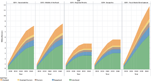
Projected cropland, cropland pasture, pasture, and forestland converting to developed land across each SSP from 2015 to 2065 in million hectares.
Projected cropland, cropland pasture, pasture, and forestland converting to developed land across each SSP from 2015 to 2065 in million hectares.
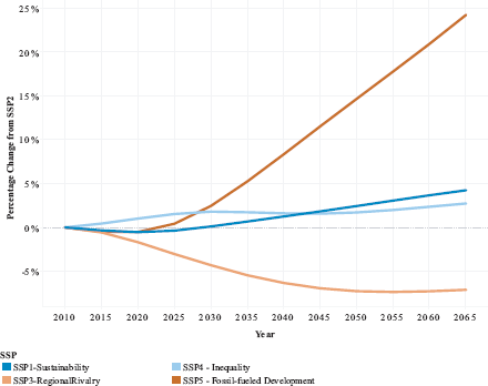
Percentage change in GDP per capita used to shift the demand curve for agricultural commodities, relative to SSP2, across the other SSP scenarios.
Percentage change in GDP per capita used to shift the demand curve for agricultural commodities, relative to SSP2, across the other SSP scenarios.
This shift in demand was calculated as the product of a percentage change in both wealth and diet preference assumptions on the domestic demand function. First, to reflect shifts in economic wealth across SSPs, we calculated the percent difference in GDP per capita relative to the SSP2 reference scenario for each of the other SSPs in 5-year timesteps until 2080. SSP2 is the chosen reference scenario for projecting deviations for other SSP scenarios as it represents the business-as-usual future. The demand curve for agricultural commodities was then shifted positively for SSPs with higher relative GDP per capita compared to SSP2, or negatively for SSPs with lower relative GDP, assuming a unit elastic income response. The influence of GDP shocks on agricultural commodity demand varied considerably across SSPs, in direction and magnitude. For instance, in SSP3 (the regional rivalry scenario), the U.S. experiences a 7.3% decrease in agricultural commodity demand in 2050 relative to the SSP2 reference. This is in stark contrast to SSP5 (the fossil fueled development scenario), in which the U.S. sees a 14.7% increase in 2050 relative to SSP2. We used the values for each SSP to shift the demand curve for all agricultural products within the modeling framework (Figure 2).
Next, we characterized changes in long-term U.S. diet preferences across SSP scenarios through additional exogenous demand shifts across grains and vegetables, and livestock product categories. The grain and vegetable category includes corn, soybean, wheat, sorghum, rice, vegetable oils, and potato products, and the livestock category includes pork, chicken, eggs, dairy products, and beef products. The anticipated shifts in diets under each SSP follow the qualitative guidance described in the literature (Westhoek et al. 2014, Bijl et al. 2017, O’Neill et al. 2017, Popp et al. 2017), and specific quantitative shifts are derived from the SSP database from Riahi et al. (2017). To represent shifts in demand for crops and livestock, we calculated the percent difference in per capita demand for each of these aggregate crop or livestock categories, relative to the SSP2 (Riahi et al. 2017). Differences in per capita demand for grain and vegetable commodities relative to SSP2 ranges from about 10% less by 2050 (SSP1 and SSP3) to 20% higher by 2050 in SSP5, and demand for livestock products ranges from 10% less by 2050 in SSP1 to 30% higher by 2050 in SSP5. Together, these shifts move the modeled demand curve out (to represent increases in demand) or contract demand to reflect dietary changes relative to SSP2. FASOMGHG endogenously chooses what quantity to produce of each commodity to maximize producer and consumer surplus under varying socioeconomic, and climate policy futures.
The model represents trade in major agricultural commodities using a spatial equilibrium sub-model. We shifted country-specific import demand of agricultural commodities to reflect each of the SSP scenarios, based on narratives in O’Neill et al. (2017). We assigned countries to low, lower-middle, upper-middle, and high-income categories according to the 2018 World Bank country characteristics (Bank 2017). In SSP1 and SSP2, O’Neill et al. (2017) describe overseas import demand for agricultural products as moderate. Thus, we applied baseline trade values, updated from FAOSTAT, USDA-FAS, and USDA-NASS (see Appendix Table 8 in Jones et al. (2019) for more detail). As SSP3 represents reduced agricultural trade flows and regionalized production, we assumed import demand will decrease for upper-middle and high-income countries by 5% and for lower-middle and low income by 10% (Jiang and O’Neill 2017, O’Neill et al. 2017). Under SSP4 food markets are global but market access is limited (O’Neill et al. 2017). Thus, under SSP4 we assume that upper-middle and high-income country import demand increases by 5% relative to the SSP2 reference, while overseas import demand remains constant. Last, we assume that strong globalization under SSP5 (O’Neill et al. 2017, Popp et al. 2017) results in a 5% increase in agricultural product import demand from all countries.
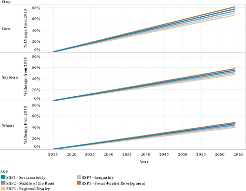
Finally, to address the different assumptions in technology growth across SSPs, we varied agricultural yield growth assumptions for each pathway (Figure 3). FASOMGHG currently incorporates dynamic yield growth assumptions for major crops as presented in Baker et al. (2013). We use the model’s baseline yield assumptions in SSP2 and assume 10% and 5% higher annual rates of yield growth under SSP5 and SSP1, respectively, following Fricko et al. (2017). On the other hand, we assume yield growth is 10% and 5% lower under SSP3 and SSP4, respectively (Fricko et al. 2017). We do not account for climate change impacts on crop yield growth across SSPs.
3.3 Forest Sector
We updated forest product demand and trade balances to reflect projected changes in trade and domestic demand. Domestic demand of forest products is based on the approach presented in Latta et al. (2018) and further developed in Jones, Baker et al. (2019). Demand elasticities for solid wood products come from Ince et al. (2011), and elasticities for shifting demand in paper products are from (Latta et al. 2015) (Table 2 in online supplementary material: Selected Mitigation Scenario Results). In the model, the domestic quantity demanded is driven by GDP, population, primary energy generation and biomass energy generation projections (Latta et al. 2018), as well as internet access estimates (Bank 2014) that drive the demand for paper and newsprint products (Latta et al. 2015), and housing starts from the 2017 Annual Energy Outlook (AEO) Reference Case (but adjusted based on population estimates for each SSP). We adopt SSP projections of population and GDP from 2015 to 2050 and then use the annual average change in GDP and population to extrapolate from 2050 to 2080. A similar approach is taken to extrapolate World Bank internet access projections beyond 2050. SSP baseline exogenous demand targets for softwood lumber and paper products are presented in Figure 4. Note that domestic demand and product prices are endogenous, but income elasticities and SSP-specific GDP projections are used to shift the projected quantity demanded for future periods.
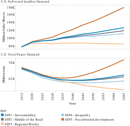
Demand curves for U.S. Softwood lumber (million m3) and paper product (million tons) across SSPs from 2015 to 2065.
Demand curves for U.S. Softwood lumber (million m3) and paper product (million tons) across SSPs from 2015 to 2065.
Changes in forest product exports are projected using results from Daigneault and Favero (2021). They used the Global Timber Model (GTM) to estimate global forest sector impacts across SSPs, which included global demand growth for pulpwood and sawlogs. We used these projections to model exogenous export demand growth across each SSP. Specifically, we start with historical export values for each forest product based on FAO (2014) (this is presented in Table 2 in Latta et al. (2018)), and then assign growth rates based on projections from Daigneault and Favero (2021). Because GTM models only pulpwood and sawtimber markets, and not individual forest products, we assigned forest products modeled in FASOMGHG to either of these categories and assumed that the growth rate for all products manufactured from sawtimber (or pulpwood) were the same. Additionally, this method assumes that the US’s relative market share to global output stays fixed over time.
3.4 Mitigation Activities
Marginal abatement costs for different abatement activities come from a variety of sources (a summary of included mitigation technologies and strategies are presented in Table 3 in online supplementary material: Selected Mitigation Scenario Results). For crop management activities such as reduced fertilization or tillage change, we have detailed crop budget data that correspond to different crops, regions, and management systems. Crop yields and emissions coefficients are linked to biogeochemical process model simulations described in Ogle et al. (2016) and Beach et al. (2010). Input use and costs are calibrated to Census of Agriculture and USDA Agricultural Resource Management Survey (ARMS) data. Mitigation activities for a single crop reflect both the direct (input cost) effect of switching management techniques and the indirect (revenue) effect of different yields. Livestock sector manure management and enteric fermentation abatement options are either represented using upward-sloping marginal abatement cost curves from (EPA 2019). Indirect mitigation can occur through reduced livestock sector production, and the model reflects these market opportunity costs. Forest management mitigation costs either reflect costs of planting or establishing a more intensive system post-harvest, the costs of thinning and other management operations, and the opportunity costs of delayed harvests. The model includes regional marginal cost curves for afforestation that correspond to different land use types, as described in Cai et al. (2018).
4 Results
Our results show that baseline GHG emissions and removals in the forest and agriculture sectors under SSP1 and SSP2 are similar, as the major difference between these two scenarios is a shift in diet preferences reducing domestic demand for meat by 10% in 2050 in SSP1 relative to SSP2 (a summary of model outputs for main forestry and agriculture commodities, as well as emissions is available in Table 1, online supplementary material). This leads to a modest increase in exports of meat products in SSP1 relative to SSP2, as we do not assume that foreign demand is reduced to the same degree as domestic demand. Importantly, the differences between these two scenarios is likely to be much larger in other sectors of the economy, due to larger differences in energy generation technology usages (Riahi et al. 2017). SSP4 results are also very similar to SSP1 and SSP2 in our analysis; globally this scenario reflects growing inequality and challenges to adaptation and mitigation measures in developing countries lagging developed countries. However, as the U.S. is a developed country, our model projections for this scenario largely reflects socioeconomic development similar to SSP1 (a scenario focused on sustainability measures, including adaptation and GHG mitigation).
Baseline emissions and removals under SSP5 are driven by large increases in population and GDP, accompanied by increased demand for both agriculture and forestry products. As a result, afforestation, forest management, agricultural intensification, and livestock herds increase in the SSP5 baseline. However, because of expanded investments in forest management and afforestation, SSP5 experiences the largest gains in baseline forest carbon sequestration and thus cumulative baseline land use sector emissions under this scenario are the smallest across all SSPs. Notably, increases in emissions from the energy sector are likely to be substantially larger under SSP5 (Bauer et al. 2017). SSP3 also results in low baseline emissions, but this is due to low population and economic growth and thus little investment in forest and agriculture sectors, as opposed to large scale investments in the forestry sector which offset agricultural emissions as in SSP5.
4.1 Differences among SSPs
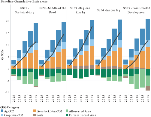
Variation across socioeconomic futures impacts baseline projections of land use, production patterns of the agriculture and forestry sectors, exports of forest and agricultural commodities, and GHG emissions (Table 1, in online supplementary material: Selected Baseline Results), are consistent with previous projections presented in Popp et al. (2017). Broadly, scenarios with higher income and demand growth show increased agriculture sector emissions over time, but also result in increased carbon sequestration in the forest sector, especially early in the simulation horizon. Although sequestration magnitudes vary across SSPs, generally the U.S. forest sector remains a carbon sink through mid-century (similar to Tian et al. (2018) and Latta et al. (2018). Agricultural sector emissions show moderate growth and some variation across SSPs, though forest carbon sequestration changes are more sensitive to our socioeconomic scenario assumptions than agricultural emissions.
SSP5, the highest demand growth scenario for both sectors, is characterized by large increases in domestic population and per capita GDP, leading to higher price growth for forest products and more investment in managed forest resources (including afforestation). This results in the most forested area and forest commodity production across all SSPs, and the highest sequestration in the early years of our analysis as investments in forest planting and management increase (shown in Figure 5). Net emissions from forests under SSP5 reach the highest levels by 2065, as harvesting ramps up to meet growing demand (net emissions are shown in Figure 6). Conversely, SSPs 3 and 4 have low population and economic growth, and therefore the least investment in afforestation, forest area, and forest commodity production, resulting in the lowest net sequestration levels from forest activities by 2065 (Figure 6). Under SSP3 we project baseline cumulative land sector GHG emissions are 43% higher than under SSP5 from 2015 to 2055, with the agricultural sector emitting 9% less emissions in SSP3 than SSP5, but the forestry sector sequestering 56% less carbon in SSP3 than SSP5 from 2015 to 2055. SSPs 1 and 2 are scenarios with moderate population and GDP growth, and therefore have middle-ground forest land use and commodity production, and thus moderate changes to projected GHG emissions. Exports of forest products vary by about 25% for pulpwood products in 2055 and nearly 40% for sawtimber products across all SSPs. For each product, SSP3 has the lowest export growth, while SSP5 has the largest increase. This export demand in SSP5 increases the relative rental rate of forest land compared to other SSPs and is a leading factor to the large forest land base found in SSP5. Cumulative forest carbon sequestration from 2015 to 2055 ranges from approximately 3.5–7.8 GtCO2e across SSPs. Results show higher sequestration levels than Latta et al. (2018) given the influence of endogenous afforestation and forest management on management.
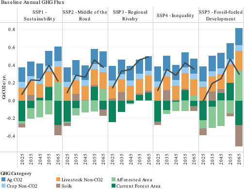
Baseline annual flux of greenhouse gases across greenhouse gas category (bars),and net annual flux (line) for each SSP from 2012 to 2065 (GtCO2e per year).
Baseline annual flux of greenhouse gases across greenhouse gas category (bars),and net annual flux (line) for each SSP from 2012 to 2065 (GtCO2e per year).
Baseline annual flux of greenhouse gases across greenhouse gas category (bars),and net annual flux (line) for each SSP from 2012 to 2065 (GtCO2e per year).
Baseline annual flux of greenhouse gases across greenhouse gas category (bars),and net annual flux (line) for each SSP from 2012 to 2065 (GtCO2e per year).
Agricultural sector emissions also vary across SSPs but are not as sensitive as changes in forest carbon sequestration. High population and income growth in SSP5, coupled with increased preference for meat products, results in agricultural intensification via increased input use (e.g., fertilizer), and increased production of corn and livestock in the U.S. This scenario also results in a slight reduction in the growth of agricultural exports relative to SSP2 as a larger share of increased production is allocated to meet domestic demand, and a relatively smaller area of land dedicated to crop, and livestock production given high relative rents from forestry seen in SSP5. This dynamic is different from the global SSP5 narrative which assumes an overall increase in agricultural trade (O’Neill et al. 2017). This scenario thus results in the highest overall emissions from agriculture among the SSPs. On the other hand, agricultural production is lowest under the low-growth SSP3, due in part to lower international demand under regional rivalry, and thus results in the lowest emissions from agriculture. SSPs 1 and 2 have moderate emissions from the
agriculture sector, due to lower population and GDP growth relative to SSP5. SSP1 has somewhat lower agricultural emissions than SSP2, with a reduction in non-CO2 emissions from livestock, driven by healthier diet assumptions including reduced meat consumption. SSP4 results in similar emissions from agriculture relative to SSPs 1 and 2, due to a combination of low population and GDP growth combined with higher exports. Across all SSPs, cumulative agriculture sector emissions range from 14.8 to 16.3 GtCO2e from 2015 to 2055.
4.2 Mitigation Potential across SSPs
We evaluate mitigation potential under a broad range of price incentives (initial mitigation prices ranging $5–$50 tCO2e-1 with 1% and 3% growth). Projections vary consistently with expectations, with higher price and higher growth mitigation incentives generating the highest levels of long-term emissions abatement, with some delayed action under higher growth scenarios due to intertemporal dynamic considerations (consistent with the findings in Baker et al. (2017), and Austin et al. (2020). We present the full set of scenarios in the online supplementary material (Figure 12) and present the $20 scenarios in the main text.
Under both of the $20tCO2e-1 scenarios (with annual growth rates of 1% and 3%), we project cumulative mitigation potentials from 2015 to 2055 that differ by more than a factor of two across SSPs (Figure 7). By 2035 we project cumulative mitigation ranging from 2.4 to 4.3 GtCO2e under SSP5 (the lowest mitigation potential across SSPs) and from 5.7 to 7.7 GtCO2e under SSP3 (the highest mitigation potential across SSPs). By 2055 mitigation increases to 8.38.8 GtCO2e under SSP5 and 17.7–20.1 GtCO2e under SSP3. These projections are roughly equivalent to annual mitigation of 200–500 million tCO2e by 2055, which is consistent with previous projections under similar carbon price assumptions and time scales (Baker et al. 2017). Our mitigation projections are generally lower than those of (Murray et al. 2005), which also used FASMGHG. These differences are partly caused by our exclusion of biofuel emissions displacement and wood product carbon storage, in addition to recent model improvements. Notably, cumulative mitigation projections are similar for the 1% and 3% scenarios even though prices are significantly higher with 3% growth. This is driven by intertemporal optimization – annual mitigation is higher under 3% growth during the last few simulation periods (2070–2080) when prices are highest, but this does not show up in our cumulative projections out to 2065 (outer years of simulation are not shown due to terminal conditions effects).
4.2.1 Forest Sector Mitigation across SSPs
Forestry activities encompass the largest share of mitigation activity across the SSPs (Figure 7). By 2055, management interventions on existing forest
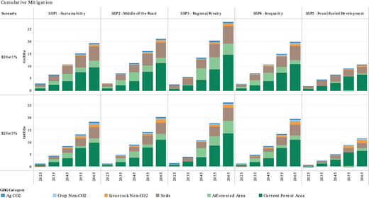
Cumulative mitigation across SSPs, under alternative mitigation price scenarios from 2025 to 2065 (GtCC>2e).
Cumulative mitigation across SSPs, under alternative mitigation price scenarios from 2025 to 2065 (GtCC>2e).
land provides the greatest source of mitigation across all SSPs within the forest sector. We project forest management to result in 44–71% of total mitigation, while afforested lands have the potential to results in net emissions due to subsequent harvesting activities under SSP5 in 2055 but are projected to contribute to cumulative mitigation in all other SSPs (Figure 7). Recent literature has focused on afforestation as an important tool for reducing GHG emissions (Bastin et al. 2019, Doelman et al. 2019, Strange et al. 2019). Our results indicate that, in the U.S. context, management change on existing forests could also provide a larger share of total mitigation potential, similar to findings in Tian et al. (2018). Forest management activities represented in the model include shifting regional harvest and production patterns, avoiding forest conversion, rotation extensions, shifting from naturally regenerated stands to planted systems, and moving to more intensive silvicultural regimes (e.g., planted forests with thinning).
Across all SSPs, we project a net forest area increase of 1.7–4.9 million hectares in the 1% growth scenario, and 1.9–4.8 hectares in the 3% scenario by 2055 relative to the no mitigation scenario (Figure 10 in online supplementary material: Selected Mitigation Scenario Results). Between 2015 and 2055, SSP5 projects increased forest plantation area of 26.2–28.5 million hectares across both growth rate scenarios, with total net forest area increasing by 24.1–26.9 million hectares. This high rate of afforestation is due to large demand for forestry products in the baseline. In 2055, demand for lumber and plywood is 55% and 13% higher in SSP5 than SSP3 (the lowest demand growth scenario), respectively, which drives forest resource investment at both the intensive (management) and extensive (afforestation) margins, even in the absence of a mitigation incentive (baseline). However, the large baseline quantity of afforestation coupled with high relative agricultural land rents in the SSP5 baseline limits the amount of additional afforestation that can occur when mitigation prices are included. This results in total forest sector mitigation potential of just 5.5 and 5.4 GtCO2e from 2015 to 2055 under the 1% and 3% growth rates, respectively (Figure 7). Of this SSP5 total mitigation, -0.2 and -0.4 GtCO2e come from afforestation and 5.6 and 5.8 GtCO2e coming from forest management from 2015 to 2055 across the 1% and 3% scenarios, respectively (Figure 11 in online supplementary material: Selected Mitigation Scenario Results).
On the other hand, under SSP3 we project low levels of baseline intensive (forest management) and extensive (afforestation) margin investments in the forest sector, due to relatively low rates of population and economic growth, which results in low rental rates of agricultural and developed land uses. However, cumulative sequestration from the current forest land base is the highest in SSP3 under no mitigation price relative to other SSPs due to reduced harvest levels and more standing timber left on the landscape. When mitigation prices are introduced, we project the highest mitigation potential from afforestation under SSP3; 4.9 GtCO2e in the 1% scenario, and 4.0 GtCO2e in the 3% scenario, from 2015 to 2055 (Figure 11 in online supplementary material), driven by the large supply of relatively low value agricultural land. Net mitigation from management of existing forests and increases in stand age is also high in SSP3 with mitigation of 8.8 and 8.5 GtCO2e stored from 2015 to 2055 in the 1% and 3% scenarios, respectively.
SSP1, SSP2, and SSP4 all result in moderate levels of mitigation through afforestation, of 1.9–2.6 GtCO2e in the 1% scenario, and 0.8-–1.3 GtCO2e from 2015 to 2055 in the 3% scenario. Increased investment in forest management under these scenarios yields 7.3–7.7 GtCO2e mitigation in the 1% scenario and 7.6–7.9 GtCO2e in the 3% scenario over the same time horizon.
4.2.2 Agricultural Mitigation across SSPs
Projected agricultural sector abatement ranges 0.5–1.1 GtCO2e in the 1% scenario and 1.1–1.3 GtCO2e in the 3% scenario (the sum of Ag CO2, Crop Non-CO2, and Livestock CO2 in Figure 7), from 2015 to 2055. This results in 5–6% of total land sector mitigation in the 1% growth scenario and 7–13% in the 3% growth scenario. Within the agriculture sector, we project changes in livestock production result in 44–64% of sector mitigation (or 3–8% of total mitigation) while changes in crop production results in 27–56% of sector mitigation (or 2–4% of total mitigation).4
Variation in agricultural sector mitigation potential is driven primarily by the differences in baseline demand for agriculture products across SSPs. SSP3 projects the highest mitigation potential of the agriculture sector, 1.1 and 1.3 GtCO2e from 2015 to 2055 in each price (Figure 7), due to low baseline demand for agricultural products, and thus lower marginal costs of abatement under a mitigation price. On the other hand, the U.S. land use sectors experiences increased pressure and higher rental rates from cropland under the SSP5 baseline, resulting in the highest marginal costs of abatement across the mitigation scenarios. Under SSP5 we project mitigation of just 0.5-–1.1 GtCO2e from 2015 to 2055 from the agricultural sector. SSPs 1, 2, and
4 show moderate levels of mitigation from the agricultural sector, achieving cumulative mitigation of 0.8–0.9 GtCO2e by 2055 in the 1% growth scenario, and 1.2–1.3 GtCO2e by 2050 in the 3% growth scenario (Figure 7).
The model selects a different portfolio of mitigation activities depending on the SSP. In SSPs 1 and 2 the most responsive activities to mitigation policies are increased manure management activities, reduction of conventional tillage, and reduction in overall cropland area. SSPs 4 and 5 rely on reduction of rice cultivation and increased manure management activities; and SSP3 also reduces rice cultivation significantly and reduces conventional tillage. Across all SSPs we project that irrigation usage will remain relatively constant, or increase. This highlights tradeoffs that will have to be made to meet growing future demand for agricultural products within a smaller agricultural land base. SSP5 sees the smallest changes to agriculture activities relative to the baseline due to the high opportunity costs tied to reduced production. This detail is shown in online supplementary material Figure 12.
It is important to note that we do not reflect relative challenges to implementing mitigation and adaptation strategies under SSPs as intended in the SSP narrative framing. This is particularly important for SSP4 (inequality) and SSP3 (regional rivalry) which both assume institutional and geopolitical challenges to achieving mitigation. It is difficult to reflect such institutional challenges within our modeling framework while harmonizing policy scenarios across the SSP baselines. Reflecting such challenges would likely reduce overall mitigation for SSP4 and SSP3 relative to our current simulation results.
4.2.3 Soils Mitigation across SSPs
Soils are another important component of the mitigation portfolio, providing 22–32% of total cumulative mitigation by mid-century. Mitigation from additional soil carbon sequestration can be attributed to both forestry and agriculture. For agriculture, soil-based mitigation comes from changes in regional crop mix strategies and choice of tillage technology – the model chooses a mix of conventional tillage, conservation tillage, and no-till options for different crops and regions.
4.2.4 Mitigation Response: Market versus Policy Drivers
We compare the contributions of demand-driven changes in forest carbon storage to policy-driven changes by calculating the cumulative forest carbon sink relative to the base year (2015) for each SSP baseline and each mitigation policy scenario. The difference in forest carbon sink levels across the baselines relative to the initial stock is solely attributable to the difference in each SSPs’ socioeconomic conditions—described below as the “demand driven carbon sink” (Figure 8). The SSPs’ baseline forest carbon accumulation between the 2015 starting period and 2055 ranges 4.8 GtCO2e to 8.6 GtCO2e in SSP3 and SSP5, respectively. This demand driven carbon sink effect is differentiated from the “mitigation policy carbon sink” effect, which is the difference in forest carbon sequestration across mitigation policy scenarios relative to each SSP baseline. The additional carbon storage incentivized by the mitigation price policy of $20tCO2e-1at 3% from 2015 to 2055 (shown in Figure 8) ranges from 5.4 GtCO2e to 12.5 GtCO2e in SSP3 and SSP5, respectively.
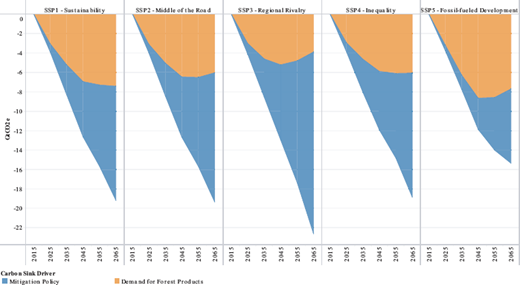
Projected change in forest carbon sink driven attributed to changes in demand for forest products (orange shaded area) under SSP assumptions, and the mitigation policy incentive (blue shaded area) in the $20@3% scenario from 2015 to 2065 (GtCO2e).
Projected change in forest carbon sink driven attributed to changes in demand for forest products (orange shaded area) under SSP assumptions, and the mitigation policy incentive (blue shaded area) in the $20@3% scenario from 2015 to 2065 (GtCO2e).
This disaggregation shows that baseline scenarios with higher levels of forest product demand growth (SSP5) show a higher rate of baseline forest carbon accumulation over time than lower growth scenarios (SSP3). Conversely, the additional net sequestration effect of a mitigation policy is muted under higher growth scenarios (SSP5). Under SSP5 and a $20tCO2e-1 at 3% price incentive, demand-driven changes in forest carbon by 2055 account for 62% of the net additional sequestration. For SSP3, this proportion is only 28% (with 72% coming from activities spurred by the price incentive). However, after mid-century, forest carbon accumulation begins to decline in all baseline SSPs, and thus the proportion of baseline forest carbon accumulation driven by socioeconomic factors decreases relative to the policy scenarios.5
Finally, our results show that as consumption of agricultural products increases so do emissions, but as consumption of forest products increases net storage of CO2 increases, and at a higher rate than agricultural sector emissions. Figure 9 presents the relationship between cumulative domestic consumption of selected commodities (softwood lumber, corn and fed beef), and GHG emissions from forestry, cropland, and livestock activities. These results indicate demand-driven changes in forest carbon accumulation offsets about 50% of increased emissions from crop and livestock systems under high emissions/high growth pathway (SSP5), but only 25% for the low growth scenario (SSP3).
5 Discussion
Land based climate change mitigation strategies are increasingly seen as critical components of limiting warming above 1.5° C to 2° C (Smith et al. 2014; Roe et al. 2019). Designing effective and cost-efficient mitigation strategies will require detailed projections of the potential magnitude of abatement activities in the forest and agriculture sectors. However, generating such projections is challenging given the magnitude of uncertainty regarding future socioeconomic trends. Therefore, producing a range of potential futures and related outcomes can help inform decision-making today. Here, we investigate the impact of alternative future scenario assumptions, represented by SSPs and alternative carbon price scenarios, on mitigation potential in the agriculture and forestry sectors. We find that the magnitude of various mitigation interventions in the forest and agriculture sectors depends on the macroeconomic context in which they are implemented. For example, we project greater mitigation potential in the SSP3 scenario, which has low economic development, (8.1–27.1 GtCO2e from 2015 to 2055, across all mitigation price scenarios, see Figure 11 in online supplementary material), as baseline investment in forests is low and there is therefore more land area available for afforestation and more opportunity for improving carbon stocks in forests via improved management under a carbon price. Conversely, the marginal cost of additional afforestation or forest management under mitigation policy scenarios is high under the SSP5, as investment in these activities is already large under the baseline. This results in projected mitigation of just 3.9–15.3 GtCO2e by 2055 under SSP5. This effect is summarized in Figure 8, which disaggregates forest carbon accumulation due to afforestation from carbon accumulation due to management changes on existing forests.
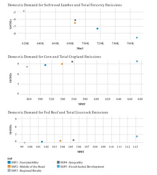
Relationships between cumulative softwood lumber demand (top), corn demand (middle), fed beef demand (bottom), and cumulative emissions under no mitigation policy scenario in 2055.
Relationships between cumulative softwood lumber demand (top), corn demand (middle), fed beef demand (bottom), and cumulative emissions under no mitigation policy scenario in 2055.
We additionally disaggregate demand- and policy-driven changes in the forest carbon stock. Management interventions driven by baseline socioeconomic conditions result in continued growth in the forest carbon sink even in the absence of a mitigation incentive. This demand-driven change in forest carbon can delay the availability of low-cost mitigation opportunities in the near-term and under low carbon prices. This finding suggests that the near-term mitigation options presented in previous literature (e.g., Fargione et al. (2018) and Haight et al. (2020)) may not be as low cost, once spatial, temporal, and sectoral market interactions are taken into consideration. This result supports the concept that policies that have contributed to the U.S. forest carbon sink (e.g., tax incentives and conservation policies) and other complementary policies (e.g., demand stimulation) could continue to encourage carbon-beneficial forest management investments.
Our findings highlight that, depending on our development trajectory, the efficient mitigation portfolio from the U.S. forest and agriculture sectors will shift. If we anticipate a high population and economic growth scenario (as in SSP5 or SSP3), it is likely that agriculture sector mitigation will be a relatively more important component of a domestic climate strategy. Whereas if we anticipate lower growth and reduced agricultural and forest product trade (as in SSP1 or SSP4), forest sector mitigation is likely to be more cost-effective. Policy makers can use insight from analyses that allow for interaction between alternative socioeconomic narratives and mitigation policy incentives to help prioritize outreach, investment, and targeted policies for reducing net emissions and bolstering sequestration from land use systems. The information systems, transaction infrastructure, and governance processes needed to facilitate forest sector mitigation may be very different from those needed for agriculture sector mitigation. For example, monitoring agriculture soils requires very different data collection processes than monitoring forest cover change (Petrokofsky et al. 2012).
Our analysis of baseline trends is unique in the context of SSPs as the U.S. is an outlier for certain SSP narratives. For example, the SSP3 scenario shows the highest levels of population growth globally along with the lowest per capita income, yet for the U.S., SSP3 has the lowest projected population growth. Similarly, SSP5 is the highest population growth scenario for the U.S., but globally SSP5 is the second-lowest population growth scenario (with SSP1 as the lowest). The U.S. is also an outlier in its high relative productivity, global market share of forest and agricultural products, and existing wealth. Subtle changes in market outputs and land use in the U.S. context can have important global implications. While FASOMGHG reflects differences in trade flows and market prices across SSPs and mitigation scenarios, the model does not simulate land use/management responses in other global regions to changes in market conditions, which may under-appreciate important feedback loops. Nonetheless, it is important for the modeling community to assess and evaluate SSP framing and scenario assumptions in their respective contexts. For this manuscript, we focused on demonstrating how SSP narratives can affect climate mitigation portfolios and costs in the agriculture and forestry sectors, though there is a need for more refined multi-stakeholder analyses of the narratives themselves and how they conform to national trends and realities. Such work can help improve SSP framing over time and could facilitate sub-national scale modeling of SSPs.
While one cannot predict what future socioeconomic pathway the U.S. and global systems will follow, our analysis provides plausible “what if” scenarios that can inform policy makers as they consider which systems and/or portfolio mixes to prioritize for land sector GHG mitigation programs. For example, if the ongoing COVID-19 pandemic results in a prolonged economic recovery period with slower growth, policy makers could consider complementary incentives (tax breaks, subsidies) to boost the forest products industry, encourage investment in the forest resource base, and increase forest carbon sequestration.
Our approach is limited in several notable ways. First, the dynamic optimization model employed for this analysis, FASOMGHG, is limited in its interactions with other sectors of the economy and impacts outside of the U.S., as it does not apply the SSPs and policy incentive outside of the U.S. land use sector. As a result, adjustments to trade flows to meet domestic demand may be over- or under-estimated. Further, FASOMGHG employs the concept that market players such as farmers and timberland managers have ‘perfect foresight’ of expected future environmental, economic, and policy conditions, which allows for optimal investment decision pathways to be determined at the cost of potentially under- or over-stating the impacts of variability in macroeconomic or policy expectations. Also, our scenarios do not account for bioenergy or other renewable energy technologies that could depend on land resources and compete with traditional agriculture and forestry commodity production.
We also note that while different SSP narratives could result in climate change impacts on agricultural systems, we do not account for potential productivity changes due to shifts in climate factors. Including climate impacts is beyond the scope of this current study and could confound the interpretation of our results that focus on the interactions between socioeconomic narrative assumptions and mitigation outcomes. However, different SSPs could result in very divergent emissions trajectories, so consideration of these long-term impacts could affect productivity rates in agriculture and forestry as well as GHG mitigation costs. Future research will attempt to explicitly link impacts and mitigation scenarios, and possibly include more linkages with global models. Finally, we acknowledge that the SSPs may underestimate uncertainty in future economic growth and low probability events that cause rapid societal change (e.g., the COVID-19 pandemic). The impact of socioeconomic (or technological) uncertainty could result in a much wider range in mitigation potential for the U.S. land use systems.
6 Conclusion
This study builds on a growing literature related to land use and GHG projections, incorporating SSP narratives into sector- and country-specific modeling applications, and quantification of land sector GHG mitigation potential and costs. Our results highlight the importance of considering alternative socioeconomic futures, which influence demand for commodities and urbanization, and impact land in forest, agriculture, livestock herds, and dependence on trade, when evaluating land use sector mitigation potential. Overall, we find that shifts in baseline assumptions around population and income growth can lead to large differences in baseline carbon fluxes and projected mitigation potential. Our results highlight the importance of putting mitigation projections in the context of assumed socioeconomic futures when designing programs aimed at limiting climate change impacts (Hoegh-Guldberg et al. 2018).
References
1 Mitigation price scenarios include initial (2020) prices of $5, $20, $35, and $50 per tCO2 equivalent and two growth rates, 1% and 3% per year, though the primary focus of the manuscript centers around the $20 scenarios.
2 Additional model documentation can be found in the online supplement.
3 The annual growth rates result in mitigation prices ranging from $90tCO2e 1 to$1,632tCO2e-1 by mid-century.
4 Figure 12 in the supplement provides additional detail on agricultural sector activities
5 Figure 13 in the supplement provides a similar graphic to Figure 8, only extended to include agricultural emissions and soil carbon sequestration. Figure 13 shows that under SSP3, changes in forest and soil carbon sequestration by 2050 relative to the base period, combined with policy-driven mitigation, outweigh the cumulative change in agricultural emissions under the baseline, but under every other SSP agricultural emissions exceed the mitigation potential.
