Contribution by J. Rimell
The contributor comments as follows regarding the paper by Thurlby (2013). The more advanced electricity distribution network operator companies currently determine condition, criticality and defect health index assessments and definitions for the majority of their infrastructure assets. In some countries, for example Great Britain (GB), asset owners are required to report to their regulator on health indices, both prior to and after their planned interventions over the regulatory planning period (8 years in the case of GB). Several of the companies use fairly sophisticated proprietary tools, such as the asset risk and prioritisation model, which improves the accuracy of the determination and prediction of asset health; these form an essential element of their asset management strategy. How does the model described in this paper compare with these existing tools, in terms of its ability to propose optimum interventions for degrading assets, that is, Opex as opposed to Capex solutions? Could the enhanced features of the model be incorporated into the models currently used by the distribution network operators (DNOs) in GB?
The recent introduction of the new regulatory scheme for the GB DNOs (RIIO-ED) has required the companies to model the effect of increased electrical loadings on the networks due to localised renewable energy take-ups – for example, electrical vehicle charging points, heat pumps and domestic- and network-embedded solar panels – and to identify optimum load-related network reinforcement solutions. The model that is generally used to perform the analyses focuses on loading capacity limitations rather than the effects of increased loadings on asset deterioration. How could the model described in the paper be developed to address any accelerated asset degradation caused by both organic load growth and more rapid load growth caused by local take-up of renewable energies?
Regulators and internal finance managers would typically expect a full cost–benefit analysis (CBA) before approving high-value schemes, using accepted cost-discount methods over the life of the asset. The output from any system dynamic modelling would be improved, and would be more acceptable to those that authorise expenditure plans, if it were to include detailed CBAs for the various options that were analysed, for example, increased maintenance intervention versus refurbishment versus replacement.
Author’s reply
The comments made by the contributor are helpful and raise some important issues which the author has attempted to address in the following discussion.
Initially it is important to recognise the role of system dynamics (SD) models in policy and strategy development. This is essentially to help planners and policy makers explore two fundamental questions.
What is likely to happen to the network if existing policies and strategies continue to be followed?
If the existing policies and strategies appear not to deliver an acceptable outcome, what are the changes that will deliver an acceptable outcome and how much will these changes cost?
System dynamics models are of most value when used to explore policy, rather than to define how policy should be implemented optimally. In short, they are best used to address the ‘what’ and ‘why’ rather than the ‘how’ and ‘which’ questions. Consequently, in the author’s view, this makes SD tools and methods complementary to other proprietary tools that can be used for asset planning. For example, an SD model developed for a UK water company concerned about the future performance of its borehole showed that, by making fundamental changes to its pump replacement and maintenance policies, operational performance would be increased and cost savings made. What the model did not do was define which individual pumps, and in what sequence, would be the subject of the new policies. This would be done with another software tool. It should be noted, however, that SD models should continue to be used to monitor the impact of the policy as it is delivered, so any changes in the dynamics can be identified and their impact mitigated by adjusting policies.
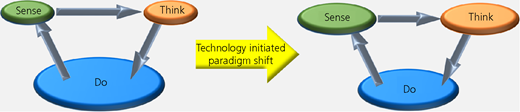
Turning to the contributor’s comment about asset health indices, this raises a fundamental challenge for all SD models, which is the availability and quality of the data required by the model. In the past, collecting and validating data could be a major challenge, especially when manual records had to be accessed and analysed. The need to create and maintain asset health indices provides a source of high-quality data that is eminently suitable for use in SD models. The problems associated with data availability and quality will be further reduced by the phenomenon of ‘big data’. Figure 10 shows how this will happen.
Traditionally, utilities and other infrastructure operators have spent most money and effort on doing work on their networks and comparatively little money and effort on measuring what was going on (sensing) and analysing the information collected (thinking) – the paradigm on the left in Figure 10. As the ‘internet of things’ becomes a reality and the cost of sensors and data storage reduces, then the amount of data available for analysis and planning will dramatically increase. In turn this will cause an explosion in analytical tools, including system dynamics, available for planning at both the policy and operational levels. Consequently, utilities and other infrastructure operators will spend much more time and effort sensing and thinking, and less time and effort doing – the paradigm on the right in Figure 10 – as they move from just doing things routinely to doing the right things at the right time.
The basic dynamics of the model has assets moving through four stages in their life; the asset ageing chain. These four stages model the changes in condition and therefore performance of the assets. In many ways these stages can be considered to be a representation of the health of the assets. It is in the design phase of model development that the different stages are defined. The condition of the assets in the network and the functionality of the model will determine this structure and the depth of detail of the ageing chain. In the majority of models there are multiple ageing chains, usually one for each major asset type. This has two advantages: first, it allows the rate of asset deterioration to be asset-type specific and so a more accurate representation of reality and, second, it enables the comparative benefits of spending Opex and Capex on individual asset types to be compared. Furthermore, an ageing chain for a single asset type may itself be split into multiple chains if there are significant differences in the operation of the assets. For example, if the model is investigating power generation assets, it would be logical to split each asset type into two ageing chains: one for those used in high-availability plant and one for those used in high-efficiency plant.
In SD models it is the rates at which assets move from one life stage to another that defines how overall condition of the infrastructure changes with time. These are known as the ‘flows’. The flow is determined by a number of factors; in the paper these factors have been simplified to maintenance and repair (Opex) and replacement/refurbishment and development (Capex). As suggested in the contributor’s comments, there are other factors, particularly how the infrastructure is used and how much it is being overloaded, which have an impact on asset degradation. These factors would be modelled as either variables or constants in the model, and become elements of the equations that define the flows. Recent development of one such model explored the capability of an infrastructure to resist and recover from disruptive events. In this case the occurrence of a disruptive event caused a flow to be immediately increased depending on the size and duration of the event. In these ways the models have the capability to address accelerated asset degradation.
Although the output of these models is often expressed as the customer minutes lost and the number of interruptions which are the result of application of a policy, particularly if the threat of an asset time bomb is being explored, it would be unusual if there was not a full cost–benefit analysis being produced for each policy as well. There is always a trade-off between the performance improvement that a policy will deliver and the cost of delivering that policy. So part of the model’s functionality is to analyse this trade-off. As infrastructure operators are invariably constrained by budgets, which they have to negotiate, it is essential that Capex and Opex expenditure for the policy that is being proposed should demonstrate that it delivers the ‘best bangs per buck’, as well as the required technical performance. SD modelling software contains the functionality to perform financial calculations, such as discounted cash flows, and it is rare that a model is built without a finance sector being part of the model.