


While many aspects of the growth mechanisms of plant roots and their ability to adapt to the surrounding environment are now clearer from a biological perspective, relatively limited research has focused on the mechanical interaction of a root and the soil in which it grows, including the root trajectory and the strain developing in the soil. The use of X-ray tomography allows for the 4D (space plus time) analysis of such an interaction. This paper investigates how plant roots grow when approaching a harder-to-penetrate soil – here, a finer and denser sand. The root trajectories in nine bilayered sand samples are imaged and characterised in terms of their tortuosity. The angle between the root axis and the gravity direction is also measured to characterise the change of trajectory of the root when approaching the stiffer sand layer. In addition, we report, for one test, the strain path experienced by the soil around the root when the latter is elongating and bending, through imaging conducted at regular intervals during the root growth.
NOTATION
INTRODUCTION
By exploring plant physics, valuable insights have been gained into the distinctive mechanics underlying growth, as well as the critical role of root system architecture in consolidation and anchorage. Through experiments focused on plant growth, scientists have been able to quantify soil deformation, analyse root–soil interaction, and develop anchorage techniques. These findings have further facilitated the creation of models that faithfully replicate the structure observed in plant roots (Sadeghi et al., 2017). At the laboratory scale, the interaction between soil and plant roots was studied under different aspects. Anselmucci et al. (2021a, 2021b) performed periodic X-ray scans on loose and dense sand samples and determined the strain field in the soil from the displacements measured by image correlation. They suggested that the increase of soil porosity near the root system is not only due to steric exclusion, as noted in previous studies, but also due to the response of the soil to shear (dilatancy). Kemp et al. (2022) observed the influence that the presence of multiple soil layers can have on the pattern of root growth. This study highlights that finer soil resulted in more linear root growth patterns, while a coarser soil granulometry caused roots to change direction towards a horizontal growth before entering the next sand layer. When plant roots encounter rigid obstacles during their growth, the accumulated force from elongation is subsequently discharged laterally, leading to slippage (Massa & Gilroy, 2003). Popova et al. (2016) characterised the tortuosity in several ways, including an index calculated from the in-plane and torsional angles. Those indices could be indicators of changes in growth response due to adaptation to the microenvironment. However, there is still limited knowledge about how roots behave when encountering a harder-to-penetrate, yet still deformable, soil.
In the present study, the soil sample consists of two sand layers, the bottom one being harder to penetrate. The objective is to study how the root that grows downward behaves when approaching, and eventually penetrating, the harder soil and to characterise strain in the soil. The growth patterns of young maize root systems in two sand layers with different grain sizes and relative densities are captured by way of X-ray tomography. Reconstructed images are analysed to investigate overall root trajectories as well as specific details such as local root orientations and soil deformations. The goal is to understand the root trajectories qualitatively and quantify the pattern of growth and the effect of root growth on the strain in the soil. Such insights help to understand the interaction between root growth and soil conditions when the surrounding environment (the soil) changes during the root growth phase. This study was carried out to inform the design of bio-inspired self-motile underground robots.
MATERIALS AND METHODS
Experiments were carried out using Hostun sand of two different grain sizes at two different relative densities. Hostun sand HN1/2·5 will be referred to as the ‘coarser sand’, and Hostun sand HN31 will be referred to as the ‘finer sand’. Table 1 presents the characteristics of the two sand types. Although Hostun sand is not representative of actual soils in which plant roots grow, it is useful as a reference for the aim of the experiment outcome.
Characteristics of the two sands used in this study. Cu = D60/D10
| Hostun sand | D50: mm | Cu | emin | emax | Dr: % |
|---|---|---|---|---|---|
| HN31 | 0·338 | 1·5 | 0·648 | 1·041 | 80 ± 4 |
| HN1-2·5 | 1·9 | 1·4 | 0·38 | 0·63 | 30 ± 11 |
The sample configuration of bilayered soil is presented in Fig. 1(a). The nine replicated bilayered soil samples consist of two layers deposited by dry pluviation, one denser layer with finer sand and a relative density of 80% ± 4%, at the bottom, and a looser layer with coarser sand and a relative density of 30% ± 11%, at the top. The two replicated single-layer soil samples consist of coarser sand only, at a relative density of 30% ± 5%. The initial properties of single-layer soil samples match the ones of top layers of bilayered soil samples. The sand is poured into a cylindrical container of 5 cm diameter and 10 cm height. The interface between the two layers is at 5 cm depth. This sample container developed by Anselmucci et al. (2021a, 2021b) has a perforated bottom that allows water to filter in but sand not to go out.
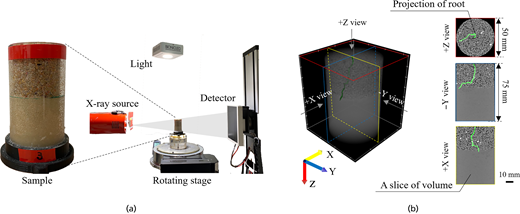
Steps for visualisation of roots; (a) data acquisition with X-ray, (b) process of visualising 3D root trajectory. To preserve 3D information, the root system is projected in three directions and coloured green. The greyscale images are obtained from a single slice at the centre of the volume and combined with the root projection. For visualisation purposes, the upper portion of the sample containing the seed and stem within the soil is cropped
Steps for visualisation of roots; (a) data acquisition with X-ray, (b) process of visualising 3D root trajectory. To preserve 3D information, the root system is projected in three directions and coloured green. The greyscale images are obtained from a single slice at the centre of the volume and combined with the root projection. For visualisation purposes, the upper portion of the sample containing the seed and stem within the soil is cropped
The root system is developed from a Zea mays L. seedling. Maize is utilised for its rapid root growth rate and its well-documented behaviour from previous experimental campaigns. The seedling is planted in the soil right after the germination of the primary root. Germination is obtained following standard procedure. The dry seed is soaked in water for 12 h, then let in a germination paper and in the dark for about 24 h prior planting the seed. The seeds are sown at a depth of 2 cm below the ground surface during the pluviation process, with the root sprout oriented downwards, and watered with fertilised water by way of capillarity, thanks to the perforated bottom. Fertiliser is mixed with distilled water at a concentration of 0·8 g/L to facilitate the root growth. The water content is equal to about 7% and to 14% in the samples with only coarser sand (the reference case) and in the bilayered samples, respectively. This is due to a difference in suction between the coarser and finer sand layers. The partially saturated samples are kept in a growing chamber with controlled temperature at 25·4°C ± 1·5°C and relative humidity at 52·9% ± 15·1%, with 14/10 h day/night cycles.
X-ray tomography and image processing
The X-ray scanner installed at Laboratoire 3SR (Grenoble) is used in this work (Viggiani et al., 2015). To ensure continuity in the plant growth, the chamber of the scanner was equipped with a radiation heater and a cold light. Quick scans with 60 µm voxel size were performed to determine whether the roots had penetrated the bottom sand layer and, if not, how far the root tips were from the boundary. Bilayered samples and single-layer samples (containing only coarse sand) were subjected to quick scans, and a bilayered sample was long-scanned with 50 µm of voxel size. Each quick scan lasted 9 min, and each long scan lasted 20 min. The latter was repeated until the roots reached the bottom sand layer. Image analyses presented in this paper were carried out with Fiji, an open-source image processing software (Schindelin et al., 2012). To investigate the strain field in the soil, the open-source python tool SPAM (Stamati et al., 2020) is used. Binarisation of the root system and segmentation of the phases were conducted following the segmentation pipeline method developed by Anselmucci et al. (2021b).
RESULTS
Global effect of two different soil layers on root growth
Figure 1(b) shows a three-dimensional (3D) reconstructed volume of the sample and the slices of the volume showing the root trajectory, the lateral walls, and the boundary between the two sand layers.
The global root trajectories obtained in all 11 samples are shown in Fig. 2. These images show the roots 4–7 days after the seeds were sown. They were scanned when the growth rate of the main root vanished in the denser sand layer. The voxel size of these images is 60 µm. After applying the bilateral and variance filters, roots were segmented and primary root trajectory was considered. In the bilayered samples, the root tip never goes deeper than 1 cm below the layer interface, resulting in a total depth of less than 6 cm. In the single sand layer, the root tips exceeded a depth of 6 cm after the same time. The bottom finer and denser sand configuration results in reduced root length, as also observed by Anselmucci et al. (2021a). In Fig. 2, two types of root trajectories can be observed: those marked with a blue asterisk, which continue growing until the primary root reaches the boundary between the two layers without touching the sidewall, and those marked with a red asterisk, which change direction and touch the sidewall. The tortuosity of each trajectory is quantified and reported at the bottom of Fig. 2 to characterise the observed 3D trajectories by means of a single scalar parameter. Tortuosity has been computed from the skeletonised images of the root limited to the region beneath the seeds. This value is the sum of the Euclidean 3D distances of the centre points of adjacent voxels in the skeletonised image divided by the Euclidean 3D linear distance from the point below the seed to the root tip. If the root is perfectly straight, the tortuosity is equal to 1, while, for instance, it is 2 if the total root length is twice the Euclidean distance. When comparing the tortuosity in the bilayered samples marked with a blue asterisk in Fig. 2, it is evident that they do not conform to a single pattern. In particular, high frequencies and large amplitudes are similarly appreciated as high tortuosity, as can be seen by comparing samples 6 and 10. This limitation has already been mentioned by Popova et al. (2016) as well. On average, the tortuosity of the root for the bilayered samples is 1·63 (blue asterisk uniquely) whereas it is 1·49 on average for the single layer samples. Although tortuosity is slightly lower in the latter case, bilayered samples cannot be clearly discriminated from single layer samples from root tortuosity only.
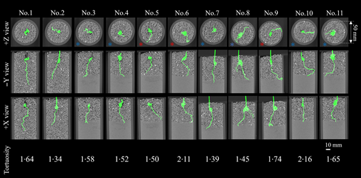
Horizontal and vertical 2D slices in the single-layer (No. 1 & 2) and bilayered samples (No. 3 to 11) 4–7 days after sowing, when the root growth rate vanished in the stiffer bottom layer. The greyscales background image shows the sand in a specific section, while the root system projection is represented in green. For the cases marked with a blue asterisk the main root continues growing until it hits the interface between the two layers without touching the sidewall, whereas for those marked with a red asterisk main root touches the sidewall. The scale-bar is reported at the bottom right
Horizontal and vertical 2D slices in the single-layer (No. 1 & 2) and bilayered samples (No. 3 to 11) 4–7 days after sowing, when the root growth rate vanished in the stiffer bottom layer. The greyscales background image shows the sand in a specific section, while the root system projection is represented in green. For the cases marked with a blue asterisk the main root continues growing until it hits the interface between the two layers without touching the sidewall, whereas for those marked with a red asterisk main root touches the sidewall. The scale-bar is reported at the bottom right
To further characterise the extent to which root growth is affected by the bottom denser sand layer, Fig. 3 shows the deviation of the root direction from the vertical (i.e. the gravity direction). The region of interest, represented by the green area below the seed (Fig. 3(a)), is skeletonised and the tangent vector A to root skeleton is computed at any point along the root. Then, the angle θ is defined as the angle between the vertical downward direction and vector A. For θ = 0 the root direction is vertical downward, for θ = 90° the root is horizontal, while θ > 90° means that the root grows upward. As an example, Fig. 3(b) shows the vertical profile of θ for sample no. 10. In Figs. 3(c) and 3(d) are shown the mean profiles of θ for all the bilayered samples and single-layer samples, respectively. The grey background represents the data range in each case. The y-axis of the graph is the vertical normalised distance L from the origin of the root, immediately under the seed, to the boundary between the two layers. In bilayered samples, the angle θ presents a global increase with depth from below the seed till the layer interface, whereas in the single-layer samples θ seems globally rather constant with depth. Furthermore, the dashed line in Fig. 3(c) represents the mean value of θ as measured in the single-layer samples – that is, it can be thought of as a ‘reference’ angle, in the absence of the bottom stiffer sand layer. This value is quite the same as the mean value for the bilayered samples for a normalised distance to the interface larger than 0·5. However, when the root approaches the boundary between the two layers, then the mean value of θ for the bilayered samples becomes larger than the reference angle, in particular for a normalised distance below 0·1, corresponding to about 3 mm, that is one to two times the mean grain size. Note that the value of θ at the interface is greater than the mean single-layer value for all nine bilayered samples.
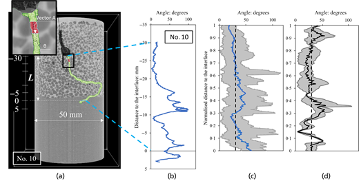
Angle θ between the direction of the root and the vertical downward direction. (a) Measurement method with the vector A tangent, at any point, to the root axis. (b) Measurement results for angle θ in sample 10. (c) Mean value of angle θ for all the bilayered samples. Grey background is the range of the data of bilayered samples. The y-axis of the graph is normalised by the distance L from the origin of the root to the boundary between the two sand layers. (d) Mean value of angle θ for all the single-layer samples. The grey background and y-axis normalisation are defined in the same way as for the bilayered soil. Single-layer samples do not have the interface between two sand layers, therefore, the mean value of L in bilayered samples is used as L in single-layer samples. The dashed lines in (c) and (d) indicate the mean value of the profiles of θ in (d) for single-layer samples
Angle θ between the direction of the root and the vertical downward direction. (a) Measurement method with the vector A tangent, at any point, to the root axis. (b) Measurement results for angle θ in sample 10. (c) Mean value of angle θ for all the bilayered samples. Grey background is the range of the data of bilayered samples. The y-axis of the graph is normalised by the distance L from the origin of the root to the boundary between the two sand layers. (d) Mean value of angle θ for all the single-layer samples. The grey background and y-axis normalisation are defined in the same way as for the bilayered soil. Single-layer samples do not have the interface between two sand layers, therefore, the mean value of L in bilayered samples is used as L in single-layer samples. The dashed lines in (c) and (d) indicate the mean value of the profiles of θ in (d) for single-layer samples
Local effect of root growth on soil strain
Sample 11 was scanned for much longer than the other samples to investigate the root–soil interaction including the change of root morphology and strain fields in soil. The long scan includes 14 scans at a constant interval of 200 min, with the first scan taken when the roots had already grown to the middle of the top coarser sand layer. Figure 4 shows some of the 14 steps analysed to illustrate the strain in the soil induced by root growth. The root penetrates the bottom sand layer between the 7th and 8th steps, 2 days after sowing the germinated seed.
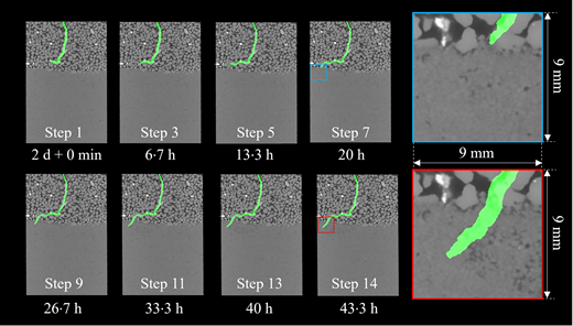
Selected central vertical slices of the 3D tomographic images of sample 11 with a constant time interval between steps and zoom-in on the interface between the two sand layers
Selected central vertical slices of the 3D tomographic images of sample 11 with a constant time interval between steps and zoom-in on the interface between the two sand layers
The strain field in the soil is obtained through 3D Digital Image Correlation. Figures 5(a) and 5(b) display the central vertical slices through the 3D volumetric and deviatoric strain fields, respectively, where the projection of the root is superimposed. Soil near the root tip predominantly dilates, as indicated by box 1 in Fig. 5(a), in the same region where higher deviatoric strains are observed (Fig. 5(b)). The soil is sheared in the vicinity of the growing root tip, and soil dilation at this location seems to be induced, at least partially, by this shearing, confirming what was found by Anselmucci et al. (2021a, 2021b) for even shorter time steps.
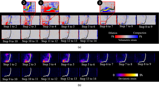
Central vertical slice through incremental strain fields for coarser-looser top sand layer decomposed into the volumetric strain (a) and the deviatoric strain (b) reach at each time increment. The root projection is superimposed as the difference between the binarised image of the root and the strain field image. Red and blue colour in (a) indicates dilation and compaction of soil, respectively
Central vertical slice through incremental strain fields for coarser-looser top sand layer decomposed into the volumetric strain (a) and the deviatoric strain (b) reach at each time increment. The root projection is superimposed as the difference between the binarised image of the root and the strain field image. Red and blue colour in (a) indicates dilation and compaction of soil, respectively
Boxes 2 and 3 in Fig. 5(a) show that soil compaction occurs in subvolumes where the root tip has already passed. These zones of compaction occur at different locations for different steps of the root growing (compare locations of boxes 2 and 3) and they seem to be positioned around root sections located before the root direction changes significantly. This suggests that the bending of the root may have influenced the deformation pattern of the surrounding soil, which typically differs from the pattern observed around the tip in previous works (Anselmucci et al., 2021a, 2021b). While soil compaction occurs in these zones, its shearing is much lower than near the tip.
To highlight the strain path experienced by the soil during the root elongation and bending, the mean total deviatoric strain in a soil subvolume is plotted in Fig. 6(a) as a function of the mean total volumetric strain in the same subvolume. The relative positions of the root with respect to this subvolume are shown in Fig. 6(b) at different times. Up to step 4, a phase of shearing with a dilative soil response (positive volumetric strain) is induced by the progression of the root tip through the subvolume. Then, from step 4 to step 8, the soil contracts at almost constant deviatoric strain, which is likely induced by the subsequent root bending. Finally, after step 8, no additional soil deformation is observed once the root tip is far enough from the subvolume.
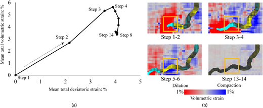
(a) Total volumetric strain (dilation is positive) in terms of total deviatoric strain averaged within the cubic subvolume where the root tip passes through with time; (b) selected central vertical slice in the incremental volumetric strain field. The cubic region of interest where the root tip passes through is superimposed in yellow with a side of 4·8 mm, which is approximately four times the diameter of the root
(a) Total volumetric strain (dilation is positive) in terms of total deviatoric strain averaged within the cubic subvolume where the root tip passes through with time; (b) selected central vertical slice in the incremental volumetric strain field. The cubic region of interest where the root tip passes through is superimposed in yellow with a side of 4·8 mm, which is approximately four times the diameter of the root
CONCLUSIONS
This study aimed to investigate the natural behaviour of plant roots as they grow in soil in the presence of a sudden change of soil stiffness and pore size. X-ray tomography was used as a non-destructive observation tool for root growth and its interaction with the two different soil layers. The results obtained from the observation of 11 samples reveal that the roots seem to be able to perceive the presence of a harder-to-penetrate sand layer, before reaching it, tending to change penetration direction. Various trajectories of roots are quantified in a single scalar parameter, tortuosity. While the sets of trajectories and tortuosities do not show a simple trend, and in spite of the large scatter of data, the measured angles between the vertical downward direction and the direction of the roots suggest an increasing trend in the bilayered samples, which is not as evident in the single-layer samples. Moreover, the root direction changes and tends to become more horizontal slightly before entering the harder-to-penetrate sand layer – at a normalised distance from it of 0·1, corresponding to about 3 mm, that is one to two times the mean grain size. Notably in this study, not only root behaviour but also soil strain was investigated, by 3D digital image correlation on images taken before and after the root penetrates the bottom sand layer. The results corroborate existing findings that soil dilation is seen around the root tip with deviatoric strain, even at a shorter time resolution than in previous studies. Nevertheless, contrary to what is observed at the root tip, after a radical change of root trajectory has occurred, soil contracts (at almost constant deviatoric strain) around root sections formed before such changes in root direction. This results in a non-monotonous strain path in the soil, which is due to root growth and bending.
Because of the inherent variability of the root–soil system, a large number of tests is clearly needed to obtain statistically representative measurements and thus draw solid conclusions about the root–soil interaction in the presence of a sharp change of resistance to penetration. However, although not necessarily representative (in a statistical sense), the results obtained in this study already provide some novel and interesting information and they shed light on some aspects of the process. These findings may lead to the development and characterisation of self-motile underground robots by mimicking the ability of plant roots to be energetically efficient, by changing their morphology and adapting their function over their lifetime in a constantly changing soil environment.
ACKNOWLEDGEMENTS
We wish to thank Pascal Charrier from 3SR for his tremendous technical help; Robert Peyroux (3SR), Barbara Mazzolai (IIT) and Emanuela Del Dottore (IIT) for very stimulating discussions, which significantly contributed to the development of this work. The first author wishes to thank Shinichiro Sawa and Takahiro Sato, both from Kumamoto University, for fruitful discussions. The first author also gratefully acknowledges the financial support from Japan Public-Private Partnership Student Study Abroad Program (TOBITATE! Young Ambassador Program). Laboratoire 3SR is part of the LabEx Tec 21 (Investissements d’Avenir – grant agreement ANR-11-LABX-0030).

