


A novel metre-scale testing concept for studying geological carbon dioxide (CO2) storage (GCS) is presented, targeting a better understanding of the interplay between the different multi-physical processes and the time scales they occur. Unlike existing laboratory- and field-scale data, the proposed intermediate scale targets high-resolution measurements while accounting for spatial distribution. A metre-scale experimental setup is designed to reproduce stress and pressure conditions similar to the field. Synthetic caprock and reservoir geomaterials are used to simulate the geological GCS layout. A first compaction and water saturation phase of the entire system is foreseen before injecting carbon dioxide in the reservoir layer, after which, an extensive post-injection monitoring period follows until total hydromechanical equilibrium. Laboratory testing and numerical modelling of the hydromechanical behaviour of the caprock/reservoir system are used to design the different phases of the proposed campaign. The metre-scale experimental results will serve as a benchmark dataset to train data-driven machine learning algorithms for improving the performance of current numerical models and future predictions in large-scale GCS.
INTRODUCTION
Geological carbon dioxide (CO2) storage (GCS) is an efficient way to store large volumes of captured carbon dioxide to meet the stringent climate goals while ensuring growing energy demand (IEA, 2022). Injecting carbon dioxide in the subsurface introduces stress changes in both the reservoir and the overlaying caprock that can result in noticeable surface deformation (uplift) (Rutqvist et al., 2008; Li & Laloui, 2016) and can cause reactivation of pre-existing faults or creation of new fractures (Rutqvist, 2012; Kim & Hosseini, 2014; Birkholzer et al., 2015). Successful upscaling of GCS requires reliable numerical models that can couple the occurring multi-physical phenomena, which manifest differently in space and time in the reservoir-caprock system (Kim & Santamarina, 2014; Pan et al., 2016; Raza et al., 2019).
Quantitative predictive models are limited due to the complexity of the emerging coupled phenomena, for example, preferential flow paths, time-dependent and temperature-induced strain and development of fractures across different spatial and temporal scales (Ilgen et al., 2017; Vilarrasa & Rutqvist, 2017). Current efforts for representative modelling are hindered by the sparse data from field-scale measurements, limited spatial resolution from well-logging techniques and the relevance of representative elementary volumes and time scales in laboratory testing (Ringrose et al., 2013; Ma et al., 2022).
In parallel, an effort to upscale with field-scale experiments is made (Manceau et al., 2015; Zappone et al., 2021; Sciandra et al., 2022); however, meaningful analysis of the acquired data requires longer monitoring time scales, so that the various space and time-dependent processes, for example, effective diffusivity, hydraulic and thermal conductivity and so on manifest. The link between the laboratory and the field is a major contemporary challenge for the development of robust GCS models.
In this work, the design of a novel approach is presented, aiming to bridge the existing lab-to-field gap in representative modelling of GCS by introducing an intermediate scale of observation. An original metre-scale testbed of the entire reservoir/caprock system is proposed to provide high-resolution measurements of the coupled geomechanical processes, while taking into account spatial variability and distribution under field representative conditions.
METHODOLOGY
Multi-scale testing is important to capture the coupled processes that take place in a wide range of scales in the caprock/reservoir system, as illustrated in Fig. 1. There are, however, unresolved challenges in successfully integrating available multi-scale data that are related to both spatial and temporal limitations. As Fig. 1 reveals, there is an important gap between existing laboratory data – which typically reach only a few centimetres – and available field data, which usually span tens of metres to kilometres. The lack of this intermediate-scale resolution makes representative upscaling less straightforward, because data integration of three orders of magnitude difference requires, on one hand, significant averaging, and on the other hand, speculative projection in time of the occurring phenomena. The methodology proposed in this work aims to enable a better understanding of the spatial and temporal interplay of the coupled processes in GCS, by introducing a unique high-resolution metre-scale dataset of the entire caprock/reservoir system (red range in Fig. 1).
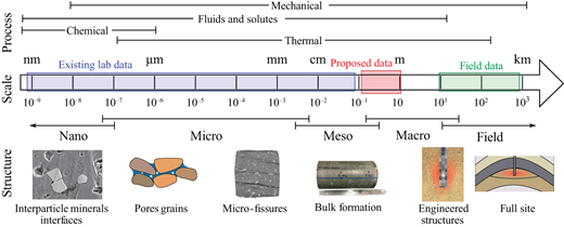
Length scales of existing data (blue and green) and targeted in this work (red), with corresponding multi-physical processes and structures relevant for GCS
Length scales of existing data (blue and green) and targeted in this work (red), with corresponding multi-physical processes and structures relevant for GCS
A metre-scale physical model for GCS
Scaled carbon dioxide injection is performed in a 1-m diameter physical model of the reservoir-caprock-overburden system. The testing setup is an original oedometer that is designed to sustain up to 20 MPa axial stress and 10 MPa fluid pressures, that is, capable to reproduce realistic GCS conditions at depths of up to 1000 m. Figure 2 shows the three-dimensional (3D) rendering of the metre-scale oedometer and a vertical two-dimensional (2D) section containing the three simulated geological layers: a reservoir layer at the bottom, a caprock layer in the middle, and an overburden formation at the top for ensuring homogeneous stress distribution on the caprock. A vertical stress is applied from the bottom with the aid of a hydraulic piston and rigid conditions are applied laterally and at the top. The pore pressure of the caprock and reservoir layers is controlled and monitored independently at two points per layer, with fluid inflow and outflow volumes also recorded at each point. The setup is designed to perform carbon dioxide injection in the reservoir as illustrated in Fig. 2.
 The image has two parts. Part a shows a cylindrical pressure vessel mounted on a steel frame. The overall height is 2.25 metres. The outer diameter is 1.20 metres and the inner diameter is 1.00 metre. Two internal vertical sections are labelled as 0.79 metres and 0.55 metres. Part b shows a cutaway schematic of the internal experimental model with a total width of 1.00 metre. The upper layer is labelled overburden with a thickness of 0.05 metres. The middle layer is labelled caprock with a thickness of 0.15 metres. The lower layer is labelled reservoir with a thickness of 0.35 metres. Carbon dioxide is injected from the top centre into the reservoir and is shown spreading outward. Optical fibre lines, pressure transducers, pore pressure and volume control units, and water connections are shown on the sides. A piston at the base applies upward axial stress, indicated by arrows.
Experimental setup: (a) 3D representation of the metre-scale oedometer with transparent cylindrical cell to display the three-layered sample; (b) vertical middle cut (red window orientation in (a)) of the setup demonstrating the hydromechanical boundary conditions and monitoring elements
The image has two parts. Part a shows a cylindrical pressure vessel mounted on a steel frame. The overall height is 2.25 metres. The outer diameter is 1.20 metres and the inner diameter is 1.00 metre. Two internal vertical sections are labelled as 0.79 metres and 0.55 metres. Part b shows a cutaway schematic of the internal experimental model with a total width of 1.00 metre. The upper layer is labelled overburden with a thickness of 0.05 metres. The middle layer is labelled caprock with a thickness of 0.15 metres. The lower layer is labelled reservoir with a thickness of 0.35 metres. Carbon dioxide is injected from the top centre into the reservoir and is shown spreading outward. Optical fibre lines, pressure transducers, pore pressure and volume control units, and water connections are shown on the sides. A piston at the base applies upward axial stress, indicated by arrows.Experimental setup: (a) 3D representation of the metre-scale oedometer with transparent cylindrical cell to display the three-layered sample; (b) vertical middle cut (red window orientation in (a)) of the setup demonstrating the hydromechanical boundary conditions and monitoring elements
Strain evolution and distribution is measured in 3D using distributed fibre optic cables (ODiSi 6000 system), providing a spatial resolution at the sub-millimetric scale (1500 points per metre) and a measurement precision of a few microns (25 ). The optical fibres are distributed within the different layers in both vertical and horizontal directions at three height and radial distance levels from the injection point, for achieving a close-to-continuous strain dataset throughout the entire setup. In addition to the optical fibres, one pressure transducer (100 kPa resolution) is installed in each layer for complementary pore pressure measurements closer to the injection point and thus, more accurate monitoring of the carbon dioxide plume propagation. Finally, the metre-scale testbed is designed to sustain temperatures up to 38°C to enable injection of both gaseous and supercritical carbon dioxide.
However, for the first validation and injection campaign, room temperature will be considered (20°C–22°C) in an effort to ensure solid control of the applied boundary conditions and the resulting HM response. Compared to the field where higher temperatures are expected in depth, injection at room temperature will not enable consideration of supercritical carbon dioxide and the study of temperature-induced couplings (e.g. pore pressure and effective stress changes). Nevertheless, the fundamental HM processes that predominantly govern structural carbon dioxide trapping during at least the first decades of storage (e.g. two-phase flow and carbon dioxide dissolution, caprock integrity and sealing response) will not be significantly altered and their study in the entire GCS system will be valuable at this resolution and scale.
Geomaterials
The targeted geological layers are simulated using synthetic caprock and reservoir geomaterials. Crushed Opalinus Clay (OPA) shale (D = 4 mm) is used to reproduce the caprock material, following a Fuller-type grain size distribution to achieve maximum density, as proposed by Fuller and Thompson (1907). The OPA shale is a material that has been broadly studied as a suitable caprock in its intact form because of its low permeability and high sealing capacity to carbon dioxide (Makhnenko et al., 2017; Stavropoulou & Laloui, 2022). The OPA used for this study originates from the Underground Research Laboratory of Mont Terri, with main mineral phases clay (54·7%), quartz (26·5%), calcite (11·3%), and siderite (5·6%), corresponding to the sandy facies (Bossart et al., 2017). The reservoir layer, typically sandstones or carbonate rocks (Vafaie et al., 2023), is reproduced using quartz sand cemented with Portland cement (0·10 gravimetric cement content). The sand-cement mixture is compacted to a target vertical stress and then saturated with water for cementation to occur during a 28-day curation period. An additional sand layer is cast over the caprock (refer to overburden in Fig. 2), to improve homogeneous stress distribution and reduce boundary-related limitations at the top of the caprock.
The caprock and reservoir geomaterials of the campaign are in granular form initially to ensure optimal distribution and contact at the lateral wall of the cell. They have been studied and designed in the laboratory (Fig. 3(a)) to reproduce to the closest the relevant mineralogical and hydromechanical properties of each natural material, that is, intact OPA shale and sandstone, respectively. In the context of GCS, a high sealing capacity and integrity is required for the caprock material. This reflects mainly in low flow properties (permeability, k) and high capillary pressures to sustain carbon dioxide entry and breakthrough (). On the contrary, the reservoir material requires high porosity and flow properties, as well as low entry pressure values to ensure high carbon dioxide injectivity.
 The image has two parts. Part a shows three cylindrical specimens placed upright. From left to right, they are labelled recompacted, O P A, and cemented sand. A vertical ruler beside the specimens provides a height reference. The O P A specimen appears dark and uniform, while the cemented sand specimen has a lighter and granular texture. Part b shows a graph with void ratio on the vertical axis and effective axial stress in kilopascals on the horizontal axis using a logarithmic scale from 10 to 100000 kilopascals. Curves represent crushed O P A sandy, intact O P A sandy, sand cement dry, and cemented sand from Arroyo et al. 2005. The crushed O P A sandy curve starts near a void ratio of about 1.05 and decreases steadily with increasing stress. The intact O P A sandy curve remains near a void ratio of about 0.20 with slight reduction. The sand cement dry and cemented sand curves show intermediate void ratios that decrease gradually as stress increases.
(a) Synthetic caprock and reservoir samples after compaction and saturation; (b) void ratio evolution with applied effective axial stress
The image has two parts. Part a shows three cylindrical specimens placed upright. From left to right, they are labelled recompacted, O P A, and cemented sand. A vertical ruler beside the specimens provides a height reference. The O P A specimen appears dark and uniform, while the cemented sand specimen has a lighter and granular texture. Part b shows a graph with void ratio on the vertical axis and effective axial stress in kilopascals on the horizontal axis using a logarithmic scale from 10 to 100000 kilopascals. Curves represent crushed O P A sandy, intact O P A sandy, sand cement dry, and cemented sand from Arroyo et al. 2005. The crushed O P A sandy curve starts near a void ratio of about 1.05 and decreases steadily with increasing stress. The intact O P A sandy curve remains near a void ratio of about 0.20 with slight reduction. The sand cement dry and cemented sand curves show intermediate void ratios that decrease gradually as stress increases.(a) Synthetic caprock and reservoir samples after compaction and saturation; (b) void ratio evolution with applied effective axial stress
EXPERIMENTAL CAMPAIGN
The experimental campaign consists of two main phases: i) compaction and water saturation of the caprock/reservoir system, and ii) carbon dioxide injection and post-injection monitoring and analysis. Each phase is designed based on material characterisation in the laboratory and full-scale numerical simulations.
Compaction and water saturation
The three geological layers are progressively compacted to a target vertical stress equal to = 18 MPa under hygroscopic drained conditions. Water saturation follows after the end of the compaction and consolidation process to reproduce field conditions. To optimise the time duration of the system’s saturation, a hydraulic gradient is applied from the bottom to the top: 3 MPa pore pressure in the reservoir layer, 1 MPa pore pressure in the caprock and open atmospheric conditions (0·1 MPa) at the top. At the end of saturation, a pore pressure equal to 2 MPa is applied to the system, resulting to 16 MPa vertical effective stress.
The hydromechanical response of the caprock and reservoir materials during compaction and water saturation has been studied in the laboratory under room temperature (20°C–22°C). The main hydromechanical properties of both geomaterials are presented in Table 1. The reported values of dry density (), void ratio (e), porosity (ϕ), oedometric modulus (), and water permeability (k) were measured at 16·0 MPa vertical effective stress (). The initial water content (w0), that is, at hygroscopic conditions and the final water content (w) at fully saturated state are additionally reported.
Main hydromechanical properties of the synthetic reservoir and caprock materials measured in the laboratory at 16 MPa effective vertical stress
| Properties | Reservoir | Caprock |
|---|---|---|
| (g/cm3) | 1·86 | 2·14 |
| w0 () | 1·5 | 3·2 |
| w () | 20·2 | 11·9 |
| e (–) | 0·46 | 0·26 |
| (–) | 0·32 | 0·19 |
| (MPa) | 242·8 | 222·6 |
| k (m2) | 3·56 × 10 | 2·65 × 10 |
| (MPa) | 0·12 | 1·50 |
Figure 3(b) shows the void ratio evolution of the synthetic geomaterials at hygroscopic state with the applied effective stress. In the same graph, the response of saturated intact OPA and cemented sand is presented for comparison. The crushed OPA presents a significantly more compressive response than the synthetic sand/cement mixture of the reservoir, resulting in half the void ratio at the target effective stress. In relation to the response of intact OPA, the final void ratio of the recompacted caprock material is higher but comparable. The response of the dry reservoir material has, as expected, a lower preconsolidation response compared to the previously cemented material studied by Arroyo et al. (2013). However, at the target effective axial stress, the final void ratio is similar.
In terms of flow-related properties, both reservoir and caprock materials have porosities comparable to relevant natural geomaterials, such as Berea sandstone (≈25%, Al-Yaseri et al., 2017) and OPA shale (<20%, Minardi et al., 2021). More importantly, the measured permeability of the synthetic materials is well within the order of magnitude of the response of the intact materials, that is, 10−16 m2 for the reservoir (Krevor et al., 2012) and 10−20–10–19 m2 for the (caprock, Kim et al., 2025).
Based on the experimental data, the compaction and saturation phases are numerically simulated with a fully coupled hydromechanical finite element method (Olivella et al., 1996; Vilarrasa et al., 2010). A 2D plain strain model has been considered with a mesh composed of 3172 triangle elements and applied boundary conditions as shown in Fig. 4. A Poisson’s ratio equal to 0·30 was considered for both caprock and reservoir layers for the numerical simulation, considering values reported for sandstone and faulted caprock (Vilarrasa & Makhnenko, 2017). Compaction to 18 MPa resulted in 51 mm total vertical displacement and negligible vertical swelling during water saturation.
 The image shows a two-dimensional numerical model domain with three horizontal layers. The top layer is labelled overburden with a thickness of 0.05 metres and a uniform applied top pressure labelled p top equal to 0.1 megapascals. Below this is a caprock layer with a thickness of 0.15 metres, bounded laterally by caprock pressure labelled p cap sub i. The bottom layer is a reservoir with a thickness of 0.35 metres and lateral reservoir pressure labelled p res sub i. A vertical injection well passes through the overburden and caprock into the reservoir, ending at an injection point. The base of the model shows a vertical stress labelled sigma v equal to 18 megapascals. The total model width is 1.00 metres. The right boundary is labelled no flow. The domain is discretised with a triangular mesh pattern across all layers.
2D plain strain model – mesh and boundary conditions during (a) compaction: caprock, p = 0·1 MPa reservoir, p = 0·1 MPa; and (b) water saturation: caprock, p = 1 MPa, reservoir p = 3 MPa
The image shows a two-dimensional numerical model domain with three horizontal layers. The top layer is labelled overburden with a thickness of 0.05 metres and a uniform applied top pressure labelled p top equal to 0.1 megapascals. Below this is a caprock layer with a thickness of 0.15 metres, bounded laterally by caprock pressure labelled p cap sub i. The bottom layer is a reservoir with a thickness of 0.35 metres and lateral reservoir pressure labelled p res sub i. A vertical injection well passes through the overburden and caprock into the reservoir, ending at an injection point. The base of the model shows a vertical stress labelled sigma v equal to 18 megapascals. The total model width is 1.00 metres. The right boundary is labelled no flow. The domain is discretised with a triangular mesh pattern across all layers.2D plain strain model – mesh and boundary conditions during (a) compaction: caprock, p = 0·1 MPa reservoir, p = 0·1 MPa; and (b) water saturation: caprock, p = 1 MPa, reservoir p = 3 MPa
After 12 h of water injection from the sides (Fig. 5(a)), a horizontal flow was observed progressing rapidly through the reservoir, due to its three orders of magnitude higher permeability compared to the caprock. Once the reservoir layer became saturated, the flow transitioned vertically into the caprock, promoting a faster and more uniform distribution (Fig. 5(b)). Figure 5(c) shows the liquid saturation at the top of each layer (as indicated by the dots in Figs. 5(a) and 5(b)). The line plot reveals a change in the slope of liquid saturation at the three control points – indicating an initial transient phase followed by a more rapid saturation. This shift marks the moment when the advancing water front spans the entire layer, enabling more efficient saturation. Modelling results suggest that the reservoir reaches full saturation within just 2 days, whereas the caprock and the overburden require ≈66 days.
 The content presents liquid saturation S l in a three-layer numerical domain with an upper layer, caprock, and reservoir. Panel a shows the saturation field at t sat equal to 12 hours with boundary pressures labelled 0.1 megapascals at the top, 1 megapascal at mid height, and 3 megapascals at the base. Panel b shows the saturation field at t sat equal to 96 hours under the same boundary conditions, with a sharp saturation front at the caprock reservoir interface. A scale indicates liquid saturation from 0 to 1. Panel c shows liquid saturation S l versus time in days from 0 to 90 for the reservoir, caprock, and upper layer, with each curve increasing from near 0 to 1 at different rates.
Water saturation of the metre-scale testbed caprock/reservoir/upper layer system: (a) liquid saturation after 12 h of water injection; (b) liquid saturation after 96 h (3 days) of water injection; (c) liquid saturation with time at the top of each layer (dots in Figs. 5(a) and 5(b))
The content presents liquid saturation S l in a three-layer numerical domain with an upper layer, caprock, and reservoir. Panel a shows the saturation field at t sat equal to 12 hours with boundary pressures labelled 0.1 megapascals at the top, 1 megapascal at mid height, and 3 megapascals at the base. Panel b shows the saturation field at t sat equal to 96 hours under the same boundary conditions, with a sharp saturation front at the caprock reservoir interface. A scale indicates liquid saturation from 0 to 1. Panel c shows liquid saturation S l versus time in days from 0 to 90 for the reservoir, caprock, and upper layer, with each curve increasing from near 0 to 1 at different rates.Water saturation of the metre-scale testbed caprock/reservoir/upper layer system: (a) liquid saturation after 12 h of water injection; (b) liquid saturation after 96 h (3 days) of water injection; (c) liquid saturation with time at the top of each layer (dots in Figs. 5(a) and 5(b))
Carbon dioxide injection
Once hydromechanical equilibrium is achieved, carbon dioxide is injected in the reservoir. Carbon dioxide is introduced at gaseous form and at initial pressure equal to the water pore pressure, that is, 2 MPa. Injection is then performed under 2 ml/min constant rate, targeting a total injected volume ≈40 l, that is equal to half the pore volume of the reservoir layer after the end of the compaction and saturation phase. The carbon dioxide injection rate (q) is calculated through normalisation from field representative rates (Q) by considering the corresponding reservoir thickness at 1 km radius of influence and injection duration as follows: , where t (days) and the injection duration and reservoir thickness at the metre-scale, T and A the injection duration (years) and reservoir thickness (m) in the field. An average injection rate equal to Mt CO2/year is generally envisaged in the field, which over 20 years and ≈200 m reservoir thickness results in normalised injection rates within the range of millilitres per minute.
Based on the experimentally assessed carbon dioxide breakthrough pressure of the reservoir material in the lab ( = 0·12 MPa), advective carbon dioxide flow in the reservoir is expected for injection pressures higher than 2·12 MPa (Table 1). Carbon dioxide injection is performed under undrained conditions at the reservoir level and at the top, and under constant pressure conditions in the caprock (2 MPa pore pressure). Figure 6 shows the liquid saturation of the system after the end of carbon dioxide injection over 360 h. The numerical simulation shows that the caprock has been able to sustain carbon dioxide breakthrough for the given boundary conditions, considering the experimentally identified breakthrough pressure equal to 1·60 MPa for the same effective stress conditions (Table 1).
 The content shows a two-dimensional numerical domain with liquid saturation S l around a vertical central injection well. Boundary pressures of 2 megapascals are applied on the left and right sides. A label at the injection point indicates q C O 2 equals 2 millilitres per minute. Liquid saturation is shown using a continuous scale from 0.30 to 1.00, where lower saturation occurs near the injection point, and higher saturation appears farther away toward the boundaries. The saturation field is symmetric about the vertical centreline and transitions smoothly outward from the injection location.
State of liquid saturation at the end of carbon dioxide injection during 360 h
The content shows a two-dimensional numerical domain with liquid saturation S l around a vertical central injection well. Boundary pressures of 2 megapascals are applied on the left and right sides. A label at the injection point indicates q C O 2 equals 2 millilitres per minute. Liquid saturation is shown using a continuous scale from 0.30 to 1.00, where lower saturation occurs near the injection point, and higher saturation appears farther away toward the boundaries. The saturation field is symmetric about the vertical centreline and transitions smoothly outward from the injection location.State of liquid saturation at the end of carbon dioxide injection during 360 h
CONCLUSIONS AND PERSPECTIVES
A new metre-scale testing concept for studying GCS is introduced aiming to provide a better understanding of the coupled multi-physical processes that occur in space and time. An original oedometer with an internal diameter equal to 1 m is designed for reproducing field-representative conditions in terms of stress, pore pressure, and geological configuration: reservoir, caprock, and overburden. The reservoir and caprock layers are simulated using synthetic granular geomaterials that have been extensively studied in the laboratory under the same levels of effective stress to define their main hydromechanical properties. Porosity, permeability, and carbon dioxide breakthrough pressure are found to be within comparable orders of magnitude with the corresponding intact reservoir and caprock materials.
To reproduce field conditions, the entire geological system is first compacted and then saturated with water. Numerical simulations of the hydromechanical response suggest that more than 2 months are required for achieving full saturation and hydromechanical equilibrium, after which, carbon dioxide injection is performed in the centre of the reservoir layer under 2 ml/min constant rate. The injected carbon dioxide is maintained within the reservoir layer; and the created overpressures prohibit breakthrough in the caprock. Carbon dioxide propagation towards the surface does not occur by means of advection; however, transport through diffusion should be better understood. The minimum and maximum carbon dioxide injection pressures are identified in the lab, to ensure both efficient injection in the reservoir and successful sealing from the caprock. A post-injection monitoring phase is foreseen to study the evolution of the system’s response in time and space until final hydromechanical equilibrium. The current methodology aims to address the following scientific questions:
How can we better understand the behaviour of a full GCS system – reservoir, caprock, and overburden – as an interconnected unit, explicitly accounting for heterogeneity and interfacial processes that are typically overlooked in existing models and experiments?
How do key parameters such as pore pressure, strain, and carbon dioxide plume migration evolve at the meter scale, and how can long-term, high-resolution measurements capture these processes effectively?
How can mechanical data (e.g. fibre optic strain and total displacement) be integrated with pressure measurements to improve the predictive reliability of traditional numerical models and newly developed machine learning tools, thereby reducing uncertainty and increasing confidence in the scalability and safety of GCS?
How can the insights gained from this work be translated into a field-applicable protocol for incorporating enhanced models into operational geological carbon sequestration projects?
ACKNOWLEDGEMENTS
This work is part of the S4S-CCUS (EPFL) and EnRUp-GCS (SI/502818, SFOE). The Authors wish to thank EPFL and the Swiss Federal Office of Energy (SFOE) for the financial support, as well as the Mont Terri underground laboratory for providing the caprock material. Additional thanks to the reviewers who helped improve the quality of the manuscript.

