The hypoplasticity model presented by the author is extremely elegant and easy to implement. It is the continuous non-linear formulation that allows for easy implementation in numerical codes, without the need to distinguish numerically between elastic and plastic regions (i.e. no conditional statements). The derivation is straightforward, so that it can easily be extended to include transverse anisotropy characteristics by only a few steps. One begins by replacing the linear isotropic tensor L (i.e. equation (1) in the original paper) with a transverse anisotropy tensor L′ to result in
where L′ is chosen to be
where ◬ and ◉ are the products of two second-order tensors, of two second-order tensors, A◬B=AilBjk(ei⊗ej⊗ek⊗el) and A◉B=AikBjl(ei⊗ej⊗ek⊗el), S=s⊗s, where s is the normal vector to the bedding plane (see Fig. 2 in Bauer et al. (2004)) and ηi are stress-dependent scalars. If the four scalar parameters η1,η2,η3 and α, together with fs, are taken as constant and the non-linear part N is ignored, conventional transverse anisotropy may be achieved.
As stated by Mašín (2004) when approaching the asymptotic state boundary surface (ASBS) the anisotropic characteristics diminish. The evolution equations suggested by Bauer et al. (2004) for ηi answer this condition
where ηi0 is the initial value of ηi. When reaching the ASBS (fd=fAd), ηi equals to 1 and, for the model to represent the isotropic state as in Mašín (2004), the constant scalar α should be taken as ν/(1−2ν). At this state the new expression degenerates into that of Mašín (2012a) (since L′=I+ν/(1−2ν)1⊗1). Following the same derivation sequence as given in the paper from equations (6) to (13), a new expression is obtained for the N tensor
As in the paper, fs is determined by an increment of unloading from a normally consolidated stress state. Since at that state L′=L, the expression of fs is identical to that presented in the paper.
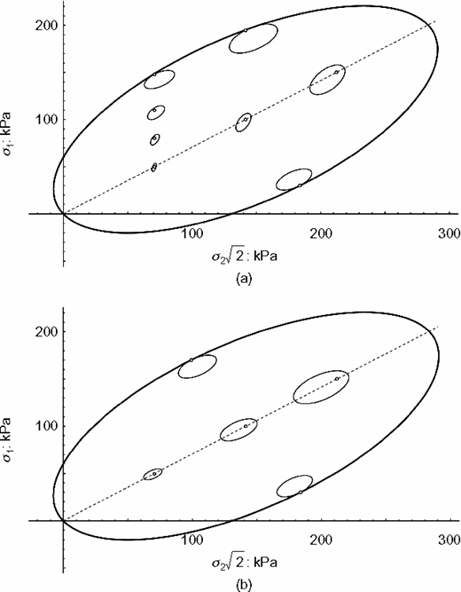
The resultant anisotropic characteristics may be investigated in the same manner as in the paper, using response envelopes. Fig. 5 shows response envelopes based on the isotropic and anisotropic models. As can be seen from Fig. 5(a), the response envelope is not symmetric about the isotropic line, as in the isotropic model (Fig. 5(b)). This directional tendency of the response envelope expresses an asymmetric tangential stiffness. As the stress state becomes closer to the ASBS, this tendency diminishes, and the response envelope resembles that of the isotropic model. The overall behaviour of the model is similar to the isotropic model, but allows certain control to characterise anisotropic features for stress states distant from the ASBS. It is believed that this may be very important for various geotechnical problems in which pre-failure anisotropy plays a major role, such as in the prediction of a settlement trough due to tunnelling (e.g. Addenbrooke et al., 1997; Puzrin et al., 2012).
Compiled dynamic-link library (DLL) files and the C++ source codes of the isotropic and anisotropic constitutive models to be used with Itasca codes (Itasca, 2009) are given by the discussers and may be downloaded from http://tx.technion.ac.il/~geo/models.
Author's reply
The author is delighted by the interest of the discussers in his research. They combined that work with the earlier results by Bauer et al. (2004) and formed a hypoplastic Cam-clay model accounting for the anisotropic response inside the state boundary surface.
Incorporation of stiffness anisotropy into hypoplasticity was, in fact, one of the motivations behind the development of the new hypoplastic approach and the author is glad that this potential of the new formulation has been recognised by the discussers. In the earlier hypoplastic models, the stiffness tensor L controlled together with N and scalar factors fs and fd the shape of the ASBS (see Mašín & Herle (2005) and Mašín (2012b)). Any modification of L thus modified also the ASBS, most likely in an undesired way. In the new approach, the ASBS can be specified independently of the formulation of the L tensor, which makes it possible to use corrected L and still have the ASBS shape under full control.
The discussers adopt a modified form of the procedure by Bauer et al. (2004), which implies that the correction of L fades away as the state approaches ASBS. This approach can be used even in combination with some earlier hypoplastic models. Full potential of the new hypoplastic approach is exploited when the anisotropic form of L is retained at the ASBS. Such a model might better represent some experimental data on clays, indicating that stiffness remains anisotropic even at higher stress ratios (Teachavorasinskun & Lukkanaprasit, 2008; Choo et al., 2011).
The approach by the discussers can still be used to construct such a model. It is merely neccesary to modify the dependency of ηi on fd (equation (28)).