
The authors have presented an interesting set of data on the comparison of elastic wave velocities measured on dry and saturated samples of granular soils and some considerations on a longitudinal pulse which has been interpreted as the longitudinal wave of the second kind (Biot-wave). The purpose of this discussion is to make a few notes that seem important in appreciating the significance of the paper.
From the comparison of the shear moduli evaluated from the shear wave velocities of dry and saturated samples, the authors conclude that the shear modulus of the saturated samples should be smaller than that of the dry sample and this could possibly be related to the wetting contacts between particles. The authors' analysis has been carried out using quite a low value of the apparent mass density: the ‘structural factor’ α has been assumed equal to 0·25 as recommended by Stoll (1989) from an investigation of the attenuation characteristics of longitudinal waves. However, there are many evaluations of the added mass density, which are based on theoretical analyses, on analogical principles and on experimental measurements (as reviewed by Gajo, 1996), which seem to show that, for granular soils comprised of round grains, the ‘tortuosity’ Τ can be approximated by
where β is the porosity and Τ = α + 1. As a consequence, the ‘structural factor’ α would be approximately equal to 0·06 for coarse Monterey sand, and approximately equal to 0·50 for medium Monterey sand and for fine crystal silica sand. These values would reduce the shear wave velocity (of about 2%) and would possibly render unnecessary the reduction of the shear modulus of saturated samples, proposed by the authors in order to have a theoretical shear wave velocity closer to the experimental data. However, these higher values of α would lead to a reduction in the computed velocity of the longitudinal waves of the second kind (about 10%) and this would change the interpretation of all the measurements. It is worth noting, however, that values of α much larger than 0·25 were used by other authors (e.g. Berryman, 1980; Van der Grinten el al., 1987) and led to a good consistency between computed and measured velocities and amplitudes of the longitudinal waves of the first and second kind.
Furthermore, the authors have observed the presence of a longitudinal pulse with an amplitude similar to or larger than the amplitude of the longitudinal wave of the first kind (P-wave). This pulse has been considered to be the longitudinal wave of the second kind (Biot-wave). The relatively large amplitude of this pulse is not consistent with theoretical evaluations of the Biot-wave, obtained using a solution based on the Laplace transform (Gajo & Mongioví, 1995) and imposing, as a driving pulse, an equal variation of the solid and fluid velocity. This boundary condition should be similar to the one imposed by the P-wave transducer used by the authors. Fig. 19 shows the distribution of effective stress, total stress and pore pressure along the direction of propagation, after a time of 100 μs.
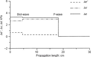
Distribution of effective stress, pore pressure and total stress, after a travel time of 100 μs, induced by a driving pulse consisting in an equal variation of the solid and fluid velocity at the boundary of a very permeable soil
Distribution of effective stress, pore pressure and total stress, after a travel time of 100 μs, induced by a driving pulse consisting in an equal variation of the solid and fluid velocity at the boundary of a very permeable soil
It can be observed that, since the solid and fluid displacements are in phase for the P-wave and out of phase for the Biot-wave, the P-wave gives an increase of both the pore pressure and the effective stress, whereas the Biot-wave leads to a decrease of the pore pressure and to an increase of the effective stress. It is worth noting that, in terms of total stress, for the assumed input parameters, the polarity of both longitudinal waves is the same, that is, the Biot-wave gives an increase of total stress. The P-wave transducer used by the authors should measure a pulse in terms of total stress and therefore the expected amplitude of the Biot-wave is very small (about 3% with respect to the amplitude of the P-wave) and the expected polarity is not consistent with the measured one. This result was obtained using the input parameters given in Table 3 for coarse Monterey sand (p′ = 79·4 kPa) and, since the damping is neglected, overestimates the real amplitude.
A longitudinal wave with such a small amplitude can be detected experimentally, but with difficulty, due to the presence of more than one longitudinal wave. In fact, in a cylindrical sample, in addition to the direct and reflected longitudinal waves of the first kind (P-waves) propagating as if the medium were infinite, there are also the longitudinal waves propagating under the influence of the lateral boundaries (E-waves). This phenomenon is well-known for the cylindrical samples consisting of one-phase material (see for instance Parton & Perlin, 1984): the higher-frequency components travel as if the medium were infinite as opposed to the lower-frequency ones, which are influenced by the lateral boundary and travel with a much lower velocity. Fig. 20 shows the results of a numerical analysis based on the finite-element method (Gajo & Mongioví, 1992) concerning the propagation of a longitudinal wave (generated by a driving pulse consisting, in a step variation, of solid and fluid velocity) along a cylindrical sample (with a diameter of 4 cm). The figure shows the wave shape (given in terms of solid velocity) after 35·53 μs, which corresponds to a travel length of the P-wave of about 1·5 diameters. It can be observed that what happens in a cylindrical sample of one-phase material holds true also for a two-phase material: there is a longitudinal wave of the first kind, travelling as if the medium were infinite (P-wave) and a slower longitudinal wave (E-wave), travelling with a velocity of about
where E is the Young's modulus of the solid skeleton and ρ is the density of the soil. If the permeability is low (Fig. 20(b)), the polarity of this slower wave (E-wave) is equal to that of the faster wave (P-wave); whereas, if permeability is high (Fig. 20(a)), the slower wave (E-wave) is confused with the long-itudinal wave of the second kind (Biot-wave) (for the elastic parameters assumed in this numerical analysis: elastic modulus E = 680 MPa, Poisson's ratio ν = 0·30, bulk moduli of the solid and of the fluid Ks = 36 GPa and Kf = 2·2 GPa, densities of solids and pore fluid ρs = 2700 kg/m3 and ρf = 1000 kg/m3, porosity β = 0·4 and tortuosity Τ = 1). This result was obtained assuming that the triaxial cell is filled with air, but the presence of water as cell fluid, due to its inertial effects, would affect in some way these results. This effect could have deeply influenced the measurements obtained by the authors, since the longitudinal pulse was observed using a low-frequency driving pulse (a single sinusoidal wave with a period of 50 μs) and filtering out the higher frequency components. A driving pulse with such a period should have given a P-wave length of about 8·5–9·5 cm, that is, probably similar to the sample height and therefore probably deeply affected by the lateral boundaries.
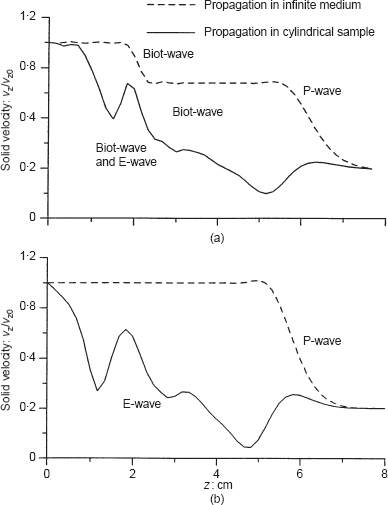
Distribution of solid velocity in an infinite medium and in a cylindrical sample, after a travel time of 35·53 μs, induced by a step variation of the solid and fluid velocity of: (a) a very permeable; and (b) an impermeable porous material (Gajo & Mongioví, 1992)
Distribution of solid velocity in an infinite medium and in a cylindrical sample, after a travel time of 35·53 μs, induced by a step variation of the solid and fluid velocity of: (a) a very permeable; and (b) an impermeable porous material (Gajo & Mongioví, 1992)
Proof of the possible difficulty in the analysis of the experimental measurements comes from the fact that the velocities of the slow E-wave (computed using equation (16)) and the input parameters (given in Table 3 by the authors) are very close to the measured velocities of the longitudinal pulse, which is assumed to be the longitudinal wave of the second kind (Biot-wave), and so the slow E-wave could have hidden the arrival of the Biot-wave. In fact, in the range of input parameters evaluated by the authors (Table 3), the velocities of the E-wave and Biot-wave are quite close to each other.
Author's reply
From the beginning of the experiment, the authors have been extremely careful about the identity of the anomalous wave found in the P-wave trace shown in Fig. 6 of the paper. In fact, as Dr Gajo discusses, it was our great concern that a cylindrical specimen used in the experiment was capable of supporting the detection of Bar-waves (termed longitudinal waves, or E-waves, by Dr Gajo). Before the publication of the paper, the possibility of the waves being Bar-waves was carefully examined. However, in order to make the paper simple, it was decided that it would not refer to bar-waves. This reply provides an opportunity for the authors to explain the reason why they consider that the anomalous P-wave is a Biot-wave and not a Bar-wave. Additional data under a different measurement configuration are also presented here in order to support their argument.
Magnitude and phase difference of the anomalous P-wave (Biot-wave)
Dr Gajo argues that the relatively large amplitude of the measured pulse of the anomalous P-wave is not consistent with the theoretical evaluations of the Biot-wave. It is worthwhile pointing out here that the theoretical calculation presented in Fig. 19 of the Discussion assumes 100% full saturation. The authors found that, when the degree of saturation became essentially 100% after applying a large back-pressure for a long period, the Biot wave was hidden by a later phase of the P-wave whose attenuation was very small. Therefore, Dr Gajo's argument is valid for 100% full saturation conditions.
As mentioned in the Discussion, the wave forms presented in Fig. 6 are obtained when the degree of saturation is slightly less than 100%, and not under the condition that Dr Gajo assumes. In order to observe the anomalous P-wave (i.e. the faster P-wave attenuates before the anomalous P-wave arrives), it was necessary to decrease the degree of saturation by varying the back-pressure. The authors explained the validity of their measurement technique using Figs 11 and 13 of the paper, which were obtained from the theoretical analysis made by Kitsunezaki (1986).
The most important feature of the anomalous P-waves in Fig. 6 of the paper is that the phase is the opposite to that of the applied pulse. The authors think that this is the unique feature of the wave, which helps to support the existence of the Biot-wave in the measured P-wave trace. When a positive motion is applied to the saturated soil, the arrival of the Biot-wave leads to a negative motion of the fluid, which the authors assume that the piezoceramic transducer is detecting. On the other hand, Dr Gajo states that the transducer will react to the changes in the total stress applied to the transducer. In this circumstance, the arrival of the Biot-wave should lead to an increase in total stress, for which the phase is the same as the input motion.
The main question that arises here is what are the characteristics of the piezoceramic transducer that detects wave motions in sand. From the experience using the piezoceramic transducers in detecting elastic wave arrivals, the authors think that the response of the transducer is not as simple as Dr Gajo explains. Piezoceramic transducers are widely used in detecting acoustic waves in liquid; for example, a hydro-phone. They are very sensitive to pressure changes in the liquid, which is in full contact with the transducer. However, when they are used in dry sand, the authors found that they are not ideal devices for detecting wave motions, possibly due to the contact condition between the transducer and soil grains. In practice, in order to detect the arrival of the P-wave in dry sand, the specimen length needed to be shortened to half (5 cm) and the wave forms had to be amplified significantly (Nakagawa el al., 1996). On the contrary, the anomalous P-waves were detected in the normal sample length of 10 cm. It is therefore difficult to believe that the transducer is detecting the grain motion in this case. The authors believe that further investigation is needed to solve this issue.
Biot-wave or Bar (or longitudinal) wave
The speed of a compressional wave in an elastic bar (Bar-wave) at the low frequency limit is given by Equation (16) in the Discussion. However, Bar waves are very dispersive and the acoustic energy is divided into various discrete modes of propagation. Each mode propagates at a speed dependent on the wave length λL, bar radius α and mode number. At low frequency, most of the energy tends to propagate in mode zero (Chotiros & Mautner, 1996). Malecki (1969) shows that, for values of α/λL less than 0·7, the zeroth mode wave speed υE may be approximated by the following equation
where E is the Young's modulus, ρ is the density, and ν is Poisson's ratio.
The Bar-wave velocities computed using equation (17) are compared with the measured Biot-wave in Fig. 21. The prediction made by Biot theory is also presented in the figure. The calculation is made for the frequency range 1–5 kHz. The dominant frequency of the measured anomalous wave generally falls into this range. The comparison is not at all to suggest that one theory is better than the other but is intended to show the whole picture of the variation of computed Bar- and Biot-wave velocities. Both theories predict similar values. However, it is worthwhile to note that the Bar-wave velocity dramatically varies within the small frequency change of 1–5 kHz.
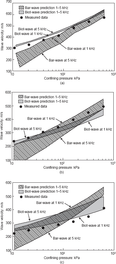
Comparison between Biot- and Bar-wave velocity predictions and measured wave velocities on: (a) coarse Monterey sand; (b) medium Monterey sand; and (c) fine silica sand
Comparison between Biot- and Bar-wave velocity predictions and measured wave velocities on: (a) coarse Monterey sand; (b) medium Monterey sand; and (c) fine silica sand
If a Bar-wave is likely to occur in the tested geometry presented in the paper, it is desirable to perform an experiment that will not allow a Bar-wave to occur. A new measurement was made in a small styroform container (220 mm (length) × 150 mm (width) × 120 mm (depth)) filled with Toyoura sand (d50 = 0·24 mm) as shown in Fig. 22. The same transducers used in the paper were buried in the container as shown in the figure. With this geometry, Bar-waves cannot occur.
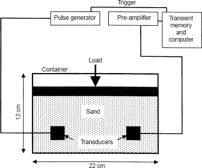
The test was done in both dry and saturated conditions. The void ratio was 0·768 for the dry sand and 0·711 for the saturated sand. A vertical load was applied on the top plate fitted to the container to provide confining pressure to the sand. The exact stress condition in the sand is rather complicated because of the presence of the transducers in the container. However, as a first approximation, it can be considered that the vertical pressure is applied uniformly to the sand.
The measured S- and P-wave traces in the dry condition are shown in Figs 23 and 24, respectively. Both velocities increase with confining pressure. The travel distance had to be smaller in this case in order to detect the feeble waves. The S- and P-wave traces in the saturated condition are shown in Figs 25 and 26, respectively. The S-wave velocity increases with confining pressure. In Fig. 26, the out-of-phase motion of the anomalous P-wave is again observed after the arrival of the fast P-wave, even though the test configuration does not allow Bar-waves to occur. In order to identify the later phase of the wave forms in Fig. 26, more clearly, the wave forms filtered by the Butterworth-type low-pass filter are shown in Fig. 27.
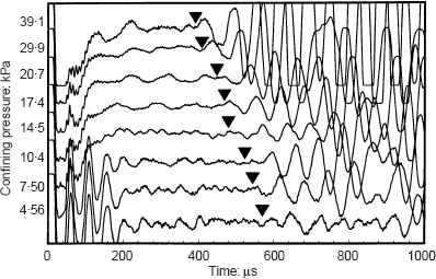
S-waveforms travelling through dry Toyoura sand. Spacing between the transducers = 7·5 cm
S-waveforms travelling through dry Toyoura sand. Spacing between the transducers = 7·5 cm
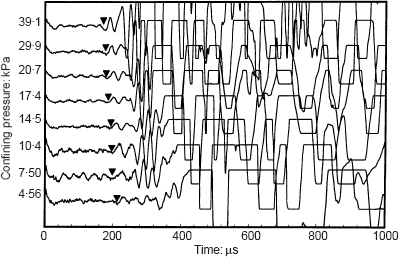
P-waveforms travelling through dry Toyoura sand. Spacing between the transducers = 7·5 cm
P-waveforms travelling through dry Toyoura sand. Spacing between the transducers = 7·5 cm
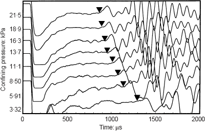
S-waveforms travelling through saturated Toyoura sand. Spacing between the transducers = 12 cm
S-waveforms travelling through saturated Toyoura sand. Spacing between the transducers = 12 cm
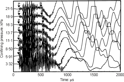
P-waveforms travelling through saturated Toyoura sand. Spacing between the transducers = 12 cm
P-waveforms travelling through saturated Toyoura sand. Spacing between the transducers = 12 cm
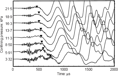
P-waveforms after using Butterworth low-pass filter on the waveforms shown in Fig. 6
P-waveforms after using Butterworth low-pass filter on the waveforms shown in Fig. 6
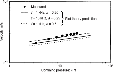
The velocities of the anomalous P-wave are compared to the computed Biot-wave velocities using equation (8) of the paper, as shown in Fig. 28. The modulus of soil skeleton was estimated from the P- and S-wave velocities measured in the dry condition, even though the saturated test had slightly denser soil than the dry test. The figure also shows the difference between the prediction using a structural factor of 0·5 rather than 0·25, as suggested by Dr Gajo. In general, the measured wave velocities are slightly larger than the predicted ones. This is possible, considering the fact that the stiffness of the soil skeleton would be larger for the saturated condition than the dry condition due to the larger density of the saturated condition. But the results are rather encouraging, supporting the authors' argument that the anomalous P-wave is likely to be the Biot-wave.
Conclusions
The authors are still in favour of the statement that the anomalous P-wave shown in Fig. 6 of the paper is the Biot-wave and not the Bar-wave. This is supported by the new data measured in a test configuration that does not allow Bar-waves to occur. However, the test results are still preliminary ones and more rigorous testing is necessary.
It is important to re-emphasize here that the arrival of the anomalous P-wave comes with an opposite motion to the applied motion. Thus, the wave is no a fast P-wave, a Bar-wave or an S-wave, which should all arrive with the same motion as the applied motion. This implies that the transducer is detecting a different wave. The numerical analysis by Dr Gajo shows that the fluid is out of phase with the soil when the slow P-wave arrives. This provides a possible explanation for the observed out-of-phase motion.
Acknowledgements
The authors would like to thank Mr Masaki Kitabayashi (Wakayama Prefectural Government) for helping the test reported in this reply, and Dr N. P. Chotiros and Ms A. M. Mautner of the University of Texas at Austin for useful comments on the paper.
