


This article examines the construction, operation and seismic performance of the El Torito tailings storage facility, Chile, under the 2015 Illapel earthquake. A two-dimensional plane strain finite-element model, employing coupled hydro-mechanical formulation, was developed to predict its response at these distinct stages. The tailings materials are simulated using a state parameter-based bounding surface plasticity model, while the remaining materials are simulated with a cyclic non-linear model. The computed seismic response of the tailings dam at the crest and the toe suggests satisfactory agreement with the monitoring data, predicting similar acceleration response spectra and spectral ratios for a wide range of periods. Limitations regarding the common lack of site-specific characterisation of tailings materials, particularly those in a decant pond, and the ensuing modelling assumptions, are also discussed. The results of this study demonstrate that advanced numerical modelling of tailings facilities to assess their safety is feasible and can be achieved if careful augmentation of the experimental data base, with studies available in the literature, is combined with appropriate engineering decisions to create a robust numerical model.
INTRODUCTION
The plethora of failure events in tailings storage facilities (TSFs) highlights the necessity to improve the general understanding of their performance. The cases of El Cobre in Chile (1965) (Dobry & Alvarez, 1967), Merriespruit in South Africa (1994) (Fourie et al., 2001), Aznalcóllar in Spain (1998) (Alonso & Gens, 2006), Mount Polley in Canada (2014) (Morgenstern et al., 2015), Fundão (2015) (Morgenstern et al., 2016) and Brumadinho (2019) (Robertson et al., 2019; Arroyo & Gens, 2021) dams in Brazil, and Cadia (2018) (Jefferies et al., 2019) in Australia are prominent examples of the severe consequences of TSFs failures. The heterogeneity of tailings materials, the complexity of the deposition and management processes, and the economic constraints of mining operators, among other factors, make these types of structures much more vulnerable to failure than a water retention dam (Davies et al., 2000). Moreover, their extensive use in highly seismic regions also renders an overall understanding of their seismic response essential. The numerical modelling of a TSF response needs to capture the material behaviour of freshly produced particles, which is not necessarily similar to that of natural soils. Consequently, the use of advanced constitutive models requires material characterisation data for calibration purposes. In the literature, tailings materials’ test data are publicly available through a limited number of research projects (e.g. Carrera et al., 2011; Li & Coop, 2019; Torres-Cruz & Santamarina, 2020; Reid et al., 2021; Macedo & Vergaray, 2022; Reid & Fanni, 2022; Russell et al., 2024) as policies of mining companies do not normally allow public dissemination of experimental data.
The term ‘tailings’ has been widely used to refer to any mine waste or residue in solid form. In geotechnical engineering, tailings can be defined as crushed rock particles, either produced or deposited in slurry form (Vick, 1990). Due to the mechanical formation processes and the usual lack of quality assurance and quality control (QA & QC) during the construction and operation of TSFs, tailings materials have inherently heterogeneous geotechnical properties. Hence, their characterisation is a difficult and underestimated task.
The modelling of TSFs through advanced constitutive models is limited in practice, especially relating to dynamic analyses, where a standard engineering practice is the use of cyclic non-linear (CNL) models coupled with conservative strength envelopes. Recent advances in constitutive models developed for natural sandy soils and their implementation in commercial finite-element (FE) and finite-difference (FD) codes have enabled their use in TSFs projects. The UBSAND model (Byrne et al., 2003) and the family of SANISAND models (Dafalias & Manzari, 2004; Taiebat & Dafalias, 2008) based on the bounding surface plasticity modelling (BSPM) framework (Manzari & Dafalias, 1997) are examples of such models. In recent years the PM4Sand (Boulanger & Ziotopoulou, 2013) model has been widely used in the simulation of earthfill dams (Boulanger & Montgomery, 2016; Boulanger, 2019), as well as TSFs (Macedo et al., 2022).
In TSF design projects, the calibration of such advanced constitutive models ideally requires a site-specific ground investigation comprising laboratory testing programmes (e.g. monotonic and cyclic triaxial tests, resonant column, cyclic direct simple shear) and in situ testing (e.g. cone penetration testing (CPT), standard penetration testing (SPT), geophysics tests). Only a few well-documented case histories are available to validate numerical simulations, based on recent failure events (e.g. Fundão in 2015 (Morgenstern et al., 2016), Brumadinho in 2019 (Robertson et al., 2019; Arroyo & Gens, 2021) and Merriespruit in 1994 (Mánica et al., 2022)). None of these cases is seismic-related, notwithstanding contrasting views suggested for Fundão (Stark et al., 2023), so well-documented seismic cases are needed in these types of dams.
The developed numerical model in the current study considers the detailed construction sequence of the El Torito tailings dam in Chile, employing coupled consolidation during its 22 years of operation and the 2015 Illapel earthquake ( = 8·3), allowing for the comparison of the dam’s response with the available monitoring data in all stages. The tailings materials are examined and calibrated employing a state parameter (Been & Jefferies, 1985) based BSPM, utilising an extensive dataset for the sand fraction. The objective is to shed light on the seismic response of tailings dams and support the use of advanced constitutive models and engineering procedures in the seismic design and assessment of this type of dams.
EL TORITO TSF
Overview
El Torito TSF in central Chile is a conventional tailings sands dam constructed using the downstream method. In the conventional method, the coarse fraction of the tailings (i.e. the tailings sands) is used to construct the dam, whereas the remaining fine fraction (i.e. fine tailings or slimes) is stored in areas constrained by the dam. The El Torito TSF is located in the highly seismic Valparaíso region and started its operation in 1993, with its construction and operation lifetime projected to 2027 (Consejo Minero, 2021). Owing to high seismicity, this TSF has suffered several earthquake events to date, including the Illapel earthquake ( = 8·3) on 16 September 2015 (Barrientos, 2015), with its epicentre 100 km away from the El Torito site. The seismic performance of the dam was satisfactory on that occasion and only negligible damage was observed (Verdugo et al., 2017). The earthquake was recorded through accelerometers at several locations on the dam.
Geology
The TSF site is characterised by sedimentary deposits, primarily alluvial to colluvial, transported by the El Cobre stream. The thickness of these sediments is unclear, but consistent with the surrounding hills and reducing as approaching the sound outcrop. Geophysical tests in 2004 (Anglo American, 2018) suggested that the maximum layer thickness varied between 80 m and 160 m. The uncertainties in the foundation layer thickness and its stiffness properties were investigated parametrically by Solans et al. (2023b).
Geometry
Due to the ‘on-going’ nature of construction and operation of TSFs, the geometric features change during their lifetime according to the storage capacity and environmental requirements. Recent data for El Torito (Consejo Minero, 2021) indicate the geometry of 13 m crest width, upstream and downstream slopes 2:1 (H:V) and 3·7:1 (H:V), respectively, while the height of 94·5 m is projected to 107 m by 2027. The operational freeboard is a minimum of 3 m and 4 m for abandonment conditions. The length of the dam varies with the development stages and was approximately 4·0 km by 2018. A plan view of the TSF is shown in Fig. 1(b).
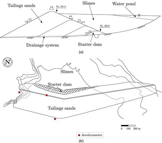
El Torito tailings dam: (a) transverse cross-section projected by 1991 (Cohen & Moenne, 1991) and (b) plan view projected by 1996 (Chilean National Committee on Large Dams, 1996)
El Torito tailings dam: (a) transverse cross-section projected by 1991 (Cohen & Moenne, 1991) and (b) plan view projected by 1996 (Chilean National Committee on Large Dams, 1996)
A drainage system consisting of a finger drain array at the dam’s base was designed to restrict the phreatic surface to approximately 5 m above the foundation level in the axis of the dam (Cohen & Moenne, 1991). The drain materials are sands and sandy gravels.
Tailings materials
The El Torito tailings sand covers a wide range of particle sizes with non-plastic fine content between 15 and 23%. Its characterisation, including critical state strength, stiffness at small strains and cyclic strength, is detailed in Solans et al. (2019) and Solans (2023). Table 1 summarises the basic properties reported for the El Torito tailings sand.
Index properties for El Torito tailings sand
| Property | El Torito tailings sand | |
|---|---|---|
| 15% FC (Solans, 2010) | 23% FC (Vargas, 2015) | |
| D50: mm | 0·16 | 0·148 |
| GS | 2·75 | 2·77 |
| CU | 3·3 | 5·72 |
| CZ | 1·2 | 1·36 |
| emax | 1·212 | 1·111 |
| emin | 0·551 | 0·462 |
The slimes are transported and stored as a slurry, generating a decant pond during the TSF construction and operation. The slimes deposition is typically not controlled, hence high heterogeneity is expected in situ, developing spatial variability of void ratio, poor shear resistance and low permeability.
GEOMETRY AND GROUND CONDITIONS
Two-dimensional plane strain time-domain FE analysis simulates the response of the El Torito TSF. The study was carried out employing the software platform ICFEP (Imperial College Finite Element Programme; Potts & Zdravković, 1999), where a hydro-mechanically (HM) coupled formulation was adopted to simulate static (construction and operation before earthquake) and dynamic stages (earthquake loading) (Kontoe, 2006; Han et al., 2016) of the dam. The time domain approach in the latter adopted the generalised-α time integration scheme (Kontoe et al., 2008).
The developed FE model is depicted in Fig. 2, with the mesh consisting of 5358 eight-noded quadrilateral isoparametric elements. The vertical element dimensions are 2 m for tailings sands, drains and starter dam, and 2 m to 4 m for slimes. In the foundation soil, vertical element dimensions of 5 m and 10 m are applied for the first 20 m and the following 60 m below the ground surface, respectively.
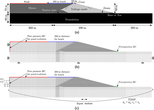
El Torito tailings dam model: (a) materials and dimensions; (b) mesh and BCs – static analysis; and (c) BCs – dynamic analysis
El Torito tailings dam model: (a) materials and dimensions; (b) mesh and BCs – static analysis; and (c) BCs – dynamic analysis
For the sake of simplicity, the geometry considered the dam crest width as 10 m, while the slope inclinations were assumed as 2:1 (H:V) and 4:1 (H:V) for the upstream and downstream faces, respectively. The suitability of lateral model dimensions and boundary conditions (BCs) was extensively examined in Solans (2023).
The mechanical BCs for the static stage are shown in Fig. 2(b), while those for the dynamic stage (Fig. 2(c)) maintained zero vertical displacements at the bottom boundary and applied tied degrees of freedom (TDOF) (Zienkiewicz et al., 1988) BC to both horizontal () and vertical () displacements along the lateral boundaries in the foundation soil. The cone BCs (Kellezi, 2000; Kontoe, 2006) were employed for the lateral vertical border of the slimes layer. The input motion was incrementally applied at the bottom model boundary as a horizontal acceleration–time history, assuming a rigid bedrock underneath.
CONSTITUTIVE MODELS
Two constitutive models are employed to simulate the mechanical behaviour of materials in the El Torito numerical model. A state parameter-based BSPM is utilised for the modelling of tailings sands (in the main dam) and slimes stored in the impoundment. The calibration process of this model for the tailings sand is detailed in Solans et al. (2023a) and will not be repeated here for brevity. The focus in this section is on the BSPM calibration for the behaviour of slimes, as these tailings materials are not usually tested in much detail that can facilitate inputs for a sophisticated constitutive model. A practical calibration approach is proposed instead and verified in the current study.
The BSPM discussion is followed by the calibration of a CNL model, which is employed to represent the foundation soil, starter dam and drains. The section completes with a discussion on the modelling of permeability, as the numerical model is HM coupled.
Bounding surface plasticity model
Tailings sand
The Taborda et al. (2014) BSPM is the base model for tailings sands and slimes, with their cyclic behaviour simulated by means of a fabric variable influencing the hardening modulus (Papadimitriou & Bouckovalas, 2002), as well as by modifications introduced by Tsaparli (2017) to the spherical part of the flow rule and to the fabric tensor, aiming to improve predictions of the cyclic strength. Further details of the model formulation and definition of parameters can be found in Taborda et al. (2014) and Tsaparli et al. (2020), the latter providing model equations for the formulation used in the current study.
Table 2 summarises the resulting model parameters for both materials. For clarification, the model parameters for the tailings sand are derived assuming 15% fines content (FC), as most of the available experiments were conducted with this FC. Solans (2023) discussed the FC effect (15% and 23%), particularly on the critical state line (CSL), and showed only slight differences in the CSL positions for the two FCs.
BSPM parameters for El Torito tailings sand and slimes
| Component | El Torito tailings sand | Slimes |
|---|---|---|
| Critical state | = 100 kPa; = 1·105; = 0·2395; = 0·205 | = 100 kPa; = 1·0; = 0·1325; = 0·135 |
| Small-strain parameters | B = 458; ng = 0·55; ν = 0·15 | B = 350; ng = 0·10; ν = 0·25 |
| Surface parameters | = 1·50; = 1·05; = 2·0; = 4·0 A0 = 0·80; A0,min = 0·0; bd = 0·10; d1 = 3·83861; d2 = 0·00538; d3 = 0·0 | = 0·983; = 0·741; = 2·0; = 4·0 A0 = 2·5; A0,min = 0·0; bd = 0·10; d1 = 0·0528; d2 = 0·01308; d3 = 0·0 |
| Hardening modulus | h0 = 0·13; = −0·10; α = 1·0; β = −0·5; γ = 0·92 | h0 = 0·10; = 0·40; α = 1·0; β = 0·0; γ = 1·10 |
| Fabric tensor | H0 = 15 000; ζ = 0·0; Cf = 75 | H0 = 0·0; ζ = 0·0; Cf = 0·0 |
Figures 3–5 are included herein to demonstrate the quality of the BSPM calibration for the tailings sand and hence facilitate the assessment of the quality and robustness of the overall El Torito numerical model. By comparing single-element FE simulations of undrained triaxial tests against experimental data, the monotonic compressions in Fig. 3, covering a large range of the mean effective stress (, from 98 kPa to 4·9 MPa) and void ratio (, from 0·613 to 0·805) values, show good reproduction of the mobilised deviatoric stress, , and phase transformation () conditions. It is worth noting that despite the high-pressure range examined experimentally, there was no evidence of particle breakage, attributed mainly to the strength of the particles (Solans, 2010). An example of a cyclic triaxial test in Fig. 4, for = 490 kPa and cyclic stress ratio, CSR = 0·250, displays similarly good agreement in terms of the cyclic stress–strain and stress-path responses. The cyclic resistance curves in Fig. 5, employing the criterion of 90% pore water pressure (PWP) build-up to define liquefaction, provide a reasonably good match with the data at around ten cycles, overestimating the cyclic strength for fewer and underestimating it for larger number of cycles. Such deviations may be explained by the inherent scatter of the data when defining the CSL and by the low initial state parameter values, , observed in the El Torito tailings sands (Solans et al., 2023a).
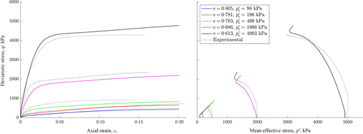
El Torito tailings sand. Simulation compared with experiments in undrained triaxial tests (data after Solans (2010))
El Torito tailings sand. Simulation compared with experiments in undrained triaxial tests (data after Solans (2010))
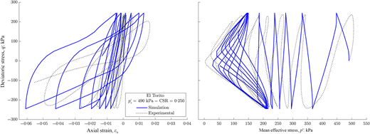
Stress–strain and stress-path responses for undrained cyclic triaxial test of the El Torito tailings sand with = 490 kPa and CSR = 0·250
Stress–strain and stress-path responses for undrained cyclic triaxial test of the El Torito tailings sand with = 490 kPa and CSR = 0·250
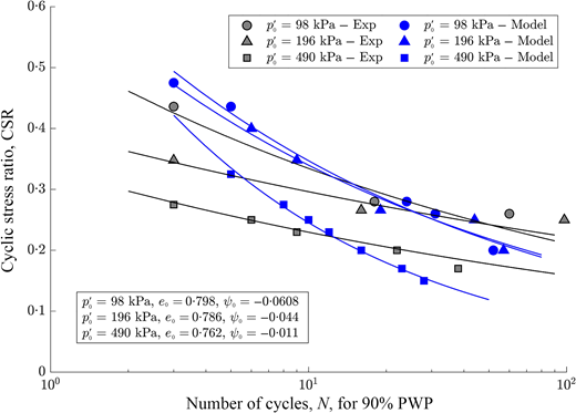
Cyclic strength curves for the El Torito tailings sand (curve fitting through power-law function) (data after Solans (2010))
Cyclic strength curves for the El Torito tailings sand (curve fitting through power-law function) (data after Solans (2010))
Tailings slimes
Owing to the high heterogeneity of slimes in situ and limited experimental data, the calibration process is focused on a practical approach that prioritises the key aspects of their behaviour: (a) strain softening from the peak undrained shear strength, ; (b) low undrained shear strength at large strains (residual), ; and (c) low cyclic resistance.
The values reported from in situ tests (Castro & Troncoso, 1989; Verdugo et al., 2014) and back-analyses of tailings dams failures (Olson & Stark, 2002; Jefferies & Been, 2016) suggest the normalised residual undrained shear strength, , in the range from 0·06 to 0·16, where is the initial in situ vertical effective stress. Expressions for obtained from experimental data were disregarded, due to the limitations in representing the in situ conditions in the laboratory for materials of this type. A target was attempted for the El Torito model. In the absence of data, the CSL for slimes is based on that defined for the tailings sand, since their mineralogy is practically the same. The adopted CSL shape, however, is closer to a straight line, compared to the curve derived for the El Torito tailings sand (Fig. 6(a)). This assumption is supported by experimental observations of Li & Coop (2019) for the Panzhihua iron tailings, China, proposing similar respective CSL shapes for fine tailings in the pond (straight line) and coarser tailings near the beach (curved). These data indicated a lower CSL gradient of the finer material than that of the coarser material. Additional supporting evidence is provided by the dataset from Jefferies & Been (2016) on tailings materials with different fine contents, indicating similar trends for the CSL slopes. The data from these two references are reproduced in the Appendix (see Figs 20 and 21 and Table 7). An alternative approach to estimating the CSL could be to adopt correlations based on the average morphology of the particles, as suggested by Lashkari et al. (2020); however, this was not considered here. The profile in Fig. 6(b) is evaluated from single-element FE simulations of triaxial compression, taking stress states in the pond area to a depth of 78 m at the end of TSF construction. The ratios of 0·1 and 0·15 are also shown as reference values, demonstrating that the profile in the numerical model is reasonably averaged by the targeted 0·1 ratio, albeit with some overestimation at depth.
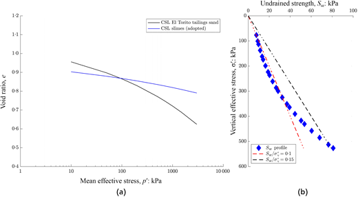
(a) Critical state line (CSL) adopted for the El Torito slimes and that calibrated for the tailings sand. (b) Undrained shear resistance profile for slimes
(a) Critical state line (CSL) adopted for the El Torito slimes and that calibrated for the tailings sand. (b) Undrained shear resistance profile for slimes
Having defined the CSL, the remaining BSPM parameters derived for the slimes which are summarised in Table 2 are: (a) low maximum shear stiffness, from the estimated S-CPT shear wave velocity ( 140 m/s, = 35 000 kPa, parameter ); (b) shear stiffness profile almost uniform with depth; (c) critical state strength envelopes with = 0·983 in compression and = 0·741 in extension ( = 25°); (d) positions of bounding ( and dilatancy () surfaces similar to the tailings sands; and (e) high dilatancy constant A0.
The performance of the adopted calibration for the El Torito slimes is depicted in terms of a monotonic undrained triaxial compression response in Fig. 7, for a range of (100–580 kPa) and void ratios (e from 0·86 to 0·90) consistent with the expected distributions in the impoundment. Highly contractant behaviour with distinct strain-softening is shown, reaching low at less than 10% axial strain. Considering the Bishop (1971) brittleness index, , as an indicator of the strain-softening response, the model simulations are in line with the overall trend for tailings materials collated by Macedo & Vergaray (2022) and reproduced in Fig. 8.
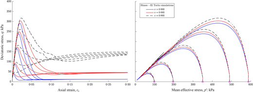
Single elements simulations for BSPM performance of slimes in undrained triaxial compression
Single elements simulations for BSPM performance of slimes in undrained triaxial compression
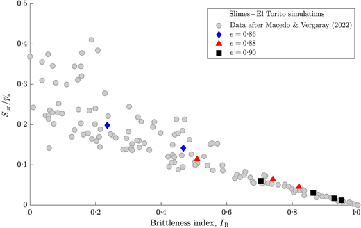
Variation of normalised residual undrained strength ratio, , plotted against , for mine tailings (data after Macedo & Vergaray (2022), compared to simulations for El Torito slimes (in coloured symbols))
Variation of normalised residual undrained strength ratio, , plotted against , for mine tailings (data after Macedo & Vergaray (2022), compared to simulations for El Torito slimes (in coloured symbols))
In the absence of site-specific data, the cyclic resistance of the slimes was based on the undrained cyclic triaxial tests on tailings materials from Ishihara et al. (1980), which include slimes’ tests from the El Cobre no. 4 TSF (same mining operation in the proximity of the El Torito TSF). The resulting cyclic resistance curves from simulations are shown in Fig. 9, adopting 85 to 90% excess PWP as a liquefaction criterion and showing a reasonably good agreement with the experimental curve derived for = 98 kPa. The calibration also examined the effect of in the cyclic response () of slimes, taking the initial values for and within the impoundment from the simulation of the construction sequence. The simulations suggested ∼ 0·5 for over 300 kPa (estimated at ten cycles), which is consistent with experimental trends observed in tailings materials (Solans, 2023).
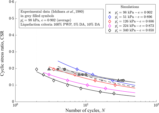
BSPM model performance for slimes under undrained cyclic triaxial conditions (curve fitting through power-law function)
BSPM model performance for slimes under undrained cyclic triaxial conditions (curve fitting through power-law function)
Cyclic non-linear model
The foundation soil, starter dam and drains are modelled with a CNL elastic model of Taborda & Zdravković (2012), coupled with a Mohr–Coulomb strength envelope. The CNL model can reproduce fundamental aspects of soil behaviour under seismic loading such as the unloading/reloading behaviour and energy dissipation through soil hysteresis.
The calibration of the CNL model typically involves evaluation of the stiffness and damping variation with strain level. Owing to the lack of experimental data for the above materials, the generic curves of Rollins et al. (1998) derived from experiments on gravels are used for calibration. The lower limit of the stiffness degradation curve suggested by Taborda & Zdravković (2012) is adopted in the model, as it introduces higher damping at very small strains, showing good agreement with the generic curve (Fig. 10). This is achieved at the expense of reproducing a lower shear stiffness at very small strains, but which is calibrated to average well the adopted generic curve over the whole small-strain range. The good fitting of the damping ratio curve is prioritised as it enables more accurate dynamic response of the dam for a broader range of strains, confirmed in simulations by Han et al. (2017) for the Kik-net downhole array. The elastic and plastic model parameters for each material are summarised in Tables 3 and 4, respectively.
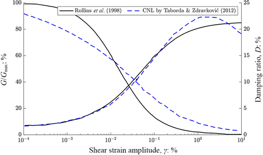
CNL model compared with empirical curves proposed by Rollins et al. (1998). Modified from Taborda & Zdravković (2012)
CNL model compared with empirical curves proposed by Rollins et al. (1998). Modified from Taborda & Zdravković (2012)
Summary CNL model parameters for the starter dam, drain and soil foundation
| Component | Starter dam / drain | Soil foundation |
|---|---|---|
| Stiffness | ||
| = 300 000 kPa; = 0·25 | = 840 000 kPa; = 0·001 | |
| = 100 kPa; = 0·25 | ||
| Shear stiffness degradation | ||
| = 5·904 × 10−5, = 0·0, = 0·0, = 1·180, = 0·03, = 10 000 kPa | ||
| Varying scaling factor | ||
| = 454·64, = 0·0, = 0·168, = 4437·21, = 0·520 | ||
Permeability models
Due to the lack of permeability data and high variability of this property in tailings materials (Mittal & Morgenstern, 1976; Vick, 1990; Valenzuela, 2015), the permeability, , was assumed isotropic in the analysis, but variable with respect to the tensile pore fluid pressure (Potts & Zdravković, 1999):
where to is a tensile PWP (suction) range over which the permeability reduces by the factor from its saturated value, . The values of model parameters are indicated in Table 5.
Permeability values employed in the analysis
| Material | Permeability, : m/s | : kPa | : kPa | |
|---|---|---|---|---|
| Tailings sand | 1·0 × 10−6 | 10 | 100 | 5 |
| Slimes | 1·0 × 10−8 | 10 | 100 | 20 |
| Foundation | — | — | — | |
| Starter dam | 5·0 × 10−6 | — | — | — |
| Drains | 1·0 × 10−5 | — | — | — |
The adopted permeability values for the tailings sands and slimes result in a phreatic surface that compares well with the position of the phreatic surface near the time of the 2015 Illapel earthquake.
INITIALISATION OF THE MODEL AND STATIC STAGE ANALYSIS
TSF construction
An approximate timeline and the downstream construction process of the TSF were simulated, resulting in the evolution of the associated initial stresses and seepage conditions in the TSF, prior to applying earthquake motion. This was achieved by first initialising the stresses in the foundation soil (, ), which is considered fully drained due to its alluvial and colluvial sediments. The construction process starts with the starter dam (dam 1 in Fig. 11(a)), followed by an alternate construction of a slimes layer (slimes 1 in Fig. 11(a)) in the decant part of the TSF, and a dam layer (dam 2), on the downstream side of the starter dam, maintaining a 2 m freeboard until reaching 80 m dam height and 78 m height of the slimes. For modelling purposes, the construction of the TSF was simplified to eight sub-stages, each stage 10 m high for both the tailings sands dam (dams 1 to 8) and the stored slimes (slimes 2 to 8), apart from slimes 1, which was 8 m high. Fig. 11(b) shows the adopted time discretisation in the construction stages. The construction process was completed in 22 years, representing the time between the start of dam construction (1993) and the recorded earthquake (2015).
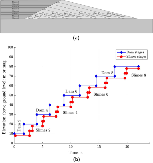
Model construction sequence (a) stage and (b) time discretisation for growing stages
Model construction sequence (a) stage and (b) time discretisation for growing stages
The evolution of the decant pond during construction and operation of the TSF is simulated with appropriate hydraulic BCs, as indicated in Fig. 2. At each construction stage a hydrostatic pore pressure (PP) BC was imposed on the newly evolved lateral boundary of the slimes, while a zero PP was applied over the top surface of the slimes, maintaining a 200 m distance to the dam as a beach. The precipitation BC (Potts & Zdravković, 2001) at the toe of the dam was applied to aid the unconfined seepage and evolution of the phreatic surface.
Upon construction, each new layer of tailings sands was prescribed an initial void ratio, e = 0·7, corresponding to a relative density ≈ 65% to 70% that is commonly observed on site for this type of TSF (Valenzuela, 2015). An initial e = 0·9 was employed for the slimes, based on the Ishihara et al. (1980) study of cyclic triaxial tests in slimes materials obtained from the same mining operation. The self-weight of the material and a prescribed suction of = 20 kPa are activated for each construction layer. The initial was calculated according to the elasticity theory (see the Poisson’s ratio, , values in Table 2).
The HM coupling was employed for the slimes, starter dam, drains and the bottom part of the tailings dam (15 m height from the base). This part of the dam was carefully studied, aiming to maintain a reasonable evolution of suction in this area due to the generated unconfined seepage flow, and to capture the resulting phreatic surface accurately. The foundation soils and the upper part of the dam were assumed drained, the latter considered appropriate for this type of problem (Boulanger, 2019) to avoid unrealistically high suctions developing if it was coupled.
Results
The results discussed here consider the end of the TSF construction, at year 22 in Fig. 11(b). Fig. 12 shows contours of the state parameter, , and of accumulated values (from the start of construction) of the resultant displacements (ABSuv), PWPs and generalised deviatoric plastic strains, . The generalised deviatoric strain is defined as
where and are the component direct and shear strains.
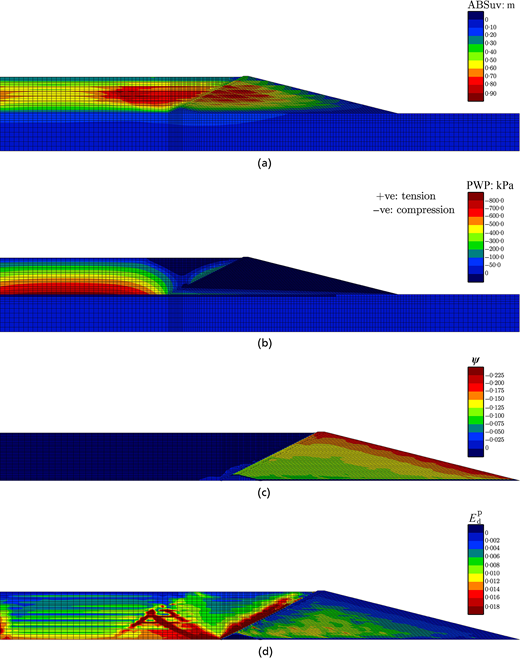
End of TSF construction, accumulated quantities: (a) resultant displacements (ABSuv); (b) pore water pressures (PWPs); (c) state parameter; (d) deviatoric plastic strain
End of TSF construction, accumulated quantities: (a) resultant displacements (ABSuv); (b) pore water pressures (PWPs); (c) state parameter; (d) deviatoric plastic strain
The displacements generated during construction (Fig. 12(a)) are mostly related to self-weight settlements, with minor contribution of horizontal displacements in the impoundment area. The maximum values are around 0·9 m close to the dam’s upstream face.
The PWP distribution in Fig. 12(b) shows the resulting phreatic surface in the dam, which reaches a height of 6 m above the ground in the dam axis, an elevation observed on site. The slimes’ PWPs are consistent with the gradual pond evolution, while the curvature in the contours indicates that excess PWPs are only partially dissipated, despite long periods of time (∼2·5 years) simulated for each construction stage. Consequently, the TSF is closer to a transient seepage rather than to a steady-state flow and the slimes at the end of the static stage can be characterised as ‘under-consolidated’, a state observed by Mittal & Morgenstern (1976) for this type of geo-structures and highly dependent on the permeability of the tailings materials.
The state parameter, , contours in Fig. 12(c) suggest mainly negative values for the tailings sands in the dam. The superficial layers are in a denser state compared to deeper layers, which are affected by the increasing during construction. In the slimes region, the state parameter is positive, , with a localised region of low negative values around the starter dam on the upstream face.
The plastic deviatoric strain, , contours indicate concentration in the impoundment (Fig. 12(d)) along the dam–slimes interface, with values of around 2%. Further shear planes are mobilised in the impoundment, associated with the geometric evolution of the pond, combined with the shear stiffness contrast. The values in the dam are lower and concentrated in its central zone, attributed to the gradual construction process, which entails small changes in the deviatoric stresses (Solans, 2023).
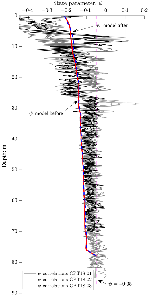
The simulation of the El Torito TSF construction and operation aimed to establish realistic stress states prior to the main seismic event in 2015. The facility has, however, also been exposed to several previous earthquakes, but without any in situ measurements it is not known how they would have altered the stress states developed by static construction. A single check of the reality of the developed construction stresses in the TSF were three CPTu tests (Anglo American, 2018) conducted along the crest of the dam 1 year after the 2015 Illapel earthquake. Fig. 13 shows CPTu-interpreted profiles of the state parameter, , below the crest, using standard methodologies of Been et al. (1987), Robertson (2010) and Shuttle & Jefferies (2016). The profile interpreted from the FE model in the centre of the crest at the end of construction agrees well with the trend of the field data, predicting gradually more dilative states on the approach to the crest. The computed profile (dashed blue line) after the 2015 Illapel earthquake is only marginally shifted to the right, indicating that prior earthquakes would not have significantly altered the predicted end of construction stresses. The dashed line ( = −0·05) is the universally accepted criterion for the onset of flow liquefaction (Shuttle & Cunning, 2008; Robertson, 2010).
SEISMIC RESPONSE
Seismic recorded data and input motion
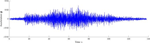
Three accelerometers located at the crest, base (toe) and an outcrop rock near the dam’s right abutment (Fig. 1(b)) recorded the 2015 Illapel earthquake ( = 8·3). Peak ground acceleration (PGA) values of 0·36 g were recorded near the epicentre (Barrientos, 2015), about 100 km away from the dam. The maximum accelerations are summarised in Table 6 for each recorded horizontal ground motion component (longitudinal and transversal) around the dam. Fig. 14 plots the resultant acceleration–time history for the transversal outcrop component, which is applied as input motion in the FE model.
Maximum acceleration values recorded at the El Torito TSF during the 2015 Illapel earthquake
| Location | Max. acceleration longitudinal: g | Max. acceleration transversal: g |
|---|---|---|
| Crest | 0·09 | 0·11 |
| Base | 0·052 | 0·05 |
| Outcrop | 0·04 | 0·03 |
Results
The seismic response of the El Torito TSF is examined in terms of the resultant displacements (ABSuv), excess PWP and deviatoric plastic strain, , at the end of the motion (Fig. 15), resulting solely from the applied motion.
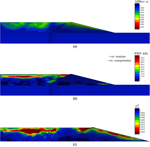
Sub-accumulated (a) resultant displacements (ABSuv), (b) excess PWP and (c) at the end of the 2015 Illapel earthquake
Sub-accumulated (a) resultant displacements (ABSuv), (b) excess PWP and (c) at the end of the 2015 Illapel earthquake
The maximum resultant displacements (Fig. 15(a)), in the dam’s downstream face, are less than 5 cm, while much smaller values are predicted in the impoundment area. The excess PWP contours (Fig. 15(b)) suggest maximum values of 50 kPa in the shallow deposits of the impoundment. Since the bottom part of the dam allows PWP build-up, there is some localised excess PWP build-up near the toe of the dam, attributed to the low values in the dam’s face. Likewise, the predicted contours in Fig. 15(c) indicate strain concentrations at shallow depths in the impoundment, with values less than 0·5%. The top part of the dam (last constructed stage) exhibits strain concentrations, which are equally small and attributed to combined effects of low and the more significant amplification observed near the dam’s surface. The part of the impoundment serving as a beach has mobilised some suctions during construction, hence experiencing limited plastic straining due to earthquake.
The predicted displacements, excess PWP and in the El Torito TSF are of low magnitude and mainly superficial. The reported ‘eye-sight’ evidence just after the earthquake indicated no damage, no permanent deformation and non-visible cracks, suggesting an excellent performance of the dam under the motion (Verdugo et al., 2017). The predicted TSF response agrees well with the reported, albeit qualitative, observations.
The computed acceleration response spectra at the crest and base of the dam in Fig. 16 are in reasonable agreement with the recorded transversal components for the whole range of frequency, capturing most of the peaks in amplitude and position. For the base of the dam, the response is well reproduced for the whole range of periods and PGA (pseudo-spectral acceleration (PSA) at = 0·01 s), while the response at the crest underestimates the PGA, with peaks of the response spectrum partly reproduced. Examining the fundamental frequencies of the model from the spectral ratio (or response amplification spectrum) of crest over base in Fig. 17, the computed response agrees well with the recorded data. Most peaks are reproduced in amplitudes and periods, except for some amplitude underestimation at very low periods and at the fundamental period estimated at 1·1 s for both spectral ratios.
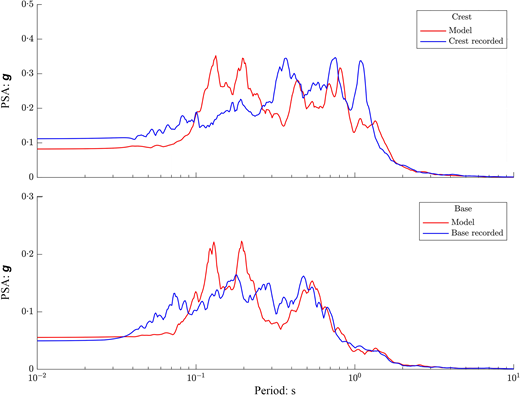
Comparison of transversal acceleration response spectra results for the El Torito tailings dam due to the 2015 Illapel earthquake
Comparison of transversal acceleration response spectra results for the El Torito tailings dam due to the 2015 Illapel earthquake
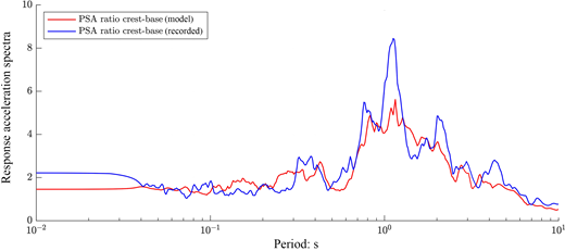
Transversal response amplification spectra comparison due to the 2015 Illapel earthquake
Transversal response amplification spectra comparison due to the 2015 Illapel earthquake
The horizontal displacements at the crest and base of the dam can be numerically integrated from the available seismic records and as such are compared with the predicted displacements (Fig. 18). It should be noted that the acceleration record at the dam’s crest was subjected to a baseline correction process due to large inferred displacements observed in the raw data. Therefore, the comparison with predicted crest displacements should be made in terms of displacement variability along the record, which is well reproduced, rather than the actual displacement magnitude. On the contrary, satisfactory agreement is obtained at the base of the model.
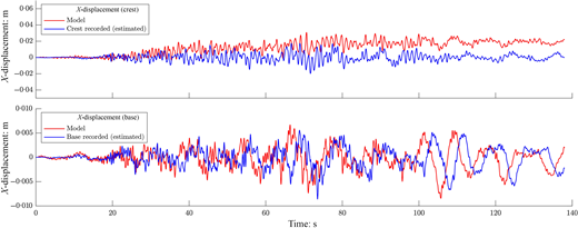
Model results and estimated recorded horizontal displacements at the crest and base of the dam due to the 2015 Illapel earthquake
Model results and estimated recorded horizontal displacements at the crest and base of the dam due to the 2015 Illapel earthquake
A final assessment herein examines the possible effect on the above comparisons of an accidental swapping of measuring directions at the crest, during the continuous change of its elevation, such that the longitudinal direction measures the transversal component and vice versa. Fig. 19(a) shows that the predicted response acceleration spectrum at the crest (taken from Fig. 16(a)) compares much more closely to the recorded longitudinal component. A similar agreement is obtained for the spectral ratio examined in Fig. 19(b). Nevertheless, by analysing theoretical and empirical approaches for determining the fundamental periods for longitudinal and transversal components (e.g. Gazetas (1981) and Park & Kishida (2019), respectively), it is not possible to determine conclusively whether the records were swapped.
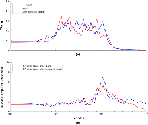
Recorded crest as longitudinal component due to the 2015 Illapel earthquake: (a) acceleration response spectra results, and (b) response amplification spectra for crest over base
Recorded crest as longitudinal component due to the 2015 Illapel earthquake: (a) acceleration response spectra results, and (b) response amplification spectra for crest over base
SUMMARY AND CONCLUSIONS
This paper examines the construction and operation of the El Torito tailings facility over a period of 22 years and its seismic response during the 2015 Illapel earthquake, employing a time-domain HM coupled FE formulation and advanced mechanical and hydraulic constitutive models. The following are key outcomes of this study.
Despite the lack of site-specific experimental data to characterise in particular the behaviour of slimes, it was possible to complement the calibration process with available studies on tailings materials in the literature and apply engineering judgement to derive representative parameters for advanced constitutive models.
In addition, the staged construction sequence developed in the FE analysis, together with appropriate hydraulic BCs to simulate the evolution of the pond area, created a robust numerical model that was effectual in reproducing realistic conditions in the facility (stresses, strains) at the end of construction, as corroborated by the comparison of the state parameter, , interpretations.
The numerical model confirmed further effectiveness in predicting a credible dynamic response of the dam under a major earthquake, as corroborated by the comparison with the available seismic records at the crest and toe of the dam.
Despite the complexity of the boundary value problem examined, the assumptions adopted and results obtained from the analysis demonstrate the feasibility of developing a robust numerical approach for assessing the life-cycle performance of tailings facilities, including those in seismic environments.
REFERENCES
Appendix
Data from Li & Coop (2019) and from Jefferies & Been (2016) can be seen in Figs 20 and 21 and Table 7.
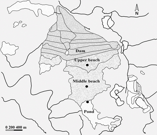
Tailings impoundment in Panzhihua: sketch of tailings impoundment with sampling locations. UP, upper beach; MB, middle beach; PO, pond (modified after Li & Coop (2019))
Tailings impoundment in Panzhihua: sketch of tailings impoundment with sampling locations. UP, upper beach; MB, middle beach; PO, pond (modified after Li & Coop (2019))
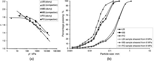
(a) Critical state lines for both reconstitution methods; (b) particle size distribution of tailings UB, MB and PO (modified after Li & Coop (2019))
(a) Critical state lines for both reconstitution methods; (b) particle size distribution of tailings UB, MB and PO (modified after Li & Coop (2019))
Experimental data for tailings materials (Jefferies & Been, 2016)
| Tailings sands and silts | D50: μm | FC: % | emax | emin | ||
|---|---|---|---|---|---|---|
| Tailings beach | 75 | 51 | 1·015 | 0·685 | 0·086 | 1·44 |
| Tailings sand | 170 | 22 | 1·065 | 0·512 | 0·115 | 1·45 |
| TCS sand | 180 | 22 | — | — | 0·115 | 1·45 |
| TCB silts | 70 | 51 | — | — | 0·086 | 1·44 |
: CSL slope in the e–log( p′) space

