


Determining earth pressure-induced moments in the active limit state is critical for the safety assessment of retaining structures. While traditional design methods assume a Coulomb's resultant force acting at one-third of the wall height, the literature suggests that the earth pressure distribution depends on the failure mode. This paper presents a rigorous kinematic solution for the ultimate moment acting on a wall undergoing rotation about its base (due to bending failure or overturning). In addition, an approximate static solution is considered. These solutions give a good approximation to the ultimate load. While the kinematic solution is closer to the exact numerical solution, the approximate static solution provides a reliable conservative approximation for common geometric and soil parameters. Its advantage is that it has a closed-form formulation. The kinematic solution is successfully validated against experimental data and is further used to investigate the peculiarities of the rotational failure mode and to evaluate traditional methods. It is found that traditional methods are close to the rigorous solutions and, therefore, reasonably safe. A useful by-product of this study: the formulation of the kinematic solution is versatile and can be applied to various geotechnical problems involving rotation.
INTRODUCTION
Quantifying the external and internal forces induced by earth pressure is essential for the design and verification of geotechnical structures. Engineers frequently calculate these forces in the ultimate limit state by assuming the active earth pressure resulting from traditional methods proposed by Coulomb (1776), Rankine (1857) or methods based on them (e.g. Poncelet, 1840; Moersch, 1925). It is common practice to use one of these solutions to derive the total earth pressure and to assume a linear pressure distribution when calculating various internal forces and moments, such as the shear force or the bending moment, regardless of the kinematics of the problem. However, several studies have shown that its distribution depends on the type of wall displacement (e.g. Tsagareli, 1965; Matsuo et al., 1978; Fang & Ishibashi, 1986), which means that the correct kinematics should be considered when verifying different types of failure (e.g. shear or bending failure).
For this reason, extensive research has been conducted to determine the earth pressure distribution depending on the wall displacement mode. For example, Terzaghi (1943) suggested that arching may cause non-linear stress distributions on retaining walls rotating about the top, a hypothesis later confirmed by empirical evidence collected by Fang & Ishibashi (1986) and extended to other displacement modes. Based on these observations, several authors proposed different approaches to quantify the earth pressure distribution. Nadukuru & Michalowski (2012) developed an analytical model using the differential slice method, which could mimic the experimental earth pressure distribution of Fang & Ishibashi (1986). However, the method needs arbitrary calibration of the mobilised friction angle along the assumed straight slip line, precluding universal practical implementation. Other authors have included the effects of soil arching in their solutions. Paik & Salgado (2003) approximated the arch shape using a circular arc to examine the pressure distribution on a wall undergoing horizontal translation. Similarly, Li et al. (2014) presented a differential slice solution considering circular arches to determine the pressure distribution behind walls rotating about the base. Patel & Deb (2020) proposed a solution including various arch shapes. However, the dependence of their solution on the wall rotation required to achieve active failure is an important issue, as it should be the outcome of a boundary value problem rather than an input parameter.
Previous research on active earth pressure has mainly focused on soil arching, but the complete wall unloading process has been overlooked. As a result, no comprehensive theory has been proposed to quantify the earth pressure for different wall displacement modes in the ultimate state. However, such a solution has been in great demand in recent years, as the condition of cantilever retaining walls in the European Alpine region has become the focus of increased attention due to corrosion revealed by destructive testing. Bending failure, characterised by the rotational movement of a wall, is the main failure mode for these structures. This has led to an extensive supranational research effort to better assess the safety of these structures (e.g. Rebhan, 2019; Haefliger & Kaufmann, 2023; Perozzi & Puzrin, 2023).
This paper is the partial result of this research effort (Perozzi & Puzrin, 2023) and uses limit analysis to investigate the ultimate load of a wall rotating about its base. First, a kinematic solution for rotational failure is formulated based on a newly introduced formulation of the energy equations for shear zones subject to linear velocity fields. The proposed kinematic solution is compared with an approximate static and a numerical limit state solution. The rigorous ultimate load derived for a rotating wall is then compared with the solution of a translational mechanism to evaluate standard design methods. In the validation stage, the kinematic solution is compared with experimental data to demonstrate the accuracy and reliability of the analysis.
PROBLEM FORMULATION AND METHODOLOGY
Figure 1 illustrates three common design scenarios in which a retaining wall experiences rotation-induced failure. To properly design the main reinforcement of a cantilever wall (depicted in Fig. 1(a)) or the profile of a sheet pile wall (Fig. 1(b)), it is necessary to quantify the bending moment, particularly at the most critical point. In the ultimate limit state, bending failure can only occur if a plastic hinge develops, resulting in an unstable system that rotates around it. This rotation causes the soil to unload, leading to active failure. In that state, the bending moment ma caused by earth pressure acts at the location of the plastic hinge. By varying the location of the plastic hinge, the engineer can obtain a distribution of the required resisting moment and optimise the design.
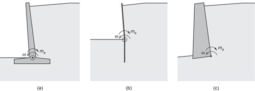
Typical geotechnical design situations: design against bending failure of (a) a cantilever retaining wall and (b) a sheet pile wall; (c) design against overturning of a gravity wall
Typical geotechnical design situations: design against bending failure of (a) a cantilever retaining wall and (b) a sheet pile wall; (c) design against overturning of a gravity wall
Similarly, the moment required to verify the stability of a wall against overturning can be determined by assuming a wall rotation about its base, as depicted in Fig. 1(c).
Under these circumstances, a bounded solution for the ultimate moment ma exerted on the wall can be determined based on the theorems of limit analysis (Drucker et al., 1952). In fact, it can be demonstrated that the actual value of the moment ma in the active ultimate state is bounded between the values determined from a kinematic and a static solution as follows
The kinematic solution relies on the commonly referenced ‘upper-bound theorem’ (as per Drucker (1954)), which delivers an upper bound of the load causing failure. However, when dealing with an active earth pressure problem, the moment ma represents the resistance that impedes failure. Therefore, in line with theorem 4 formulated by Drucker et al. (1952), it can be inferred that the kinematic solution represents an unconservative lower bound of the exact solution. Conversely, the static solution provides a conservative upper bound.
In the following, a dry, cohesionless granular soil is considered.
KINEMATIC SOLUTION
Consider the wall of height H and inclined by the angle α to the vertical depicted in Fig. 2(a), which supports a granular backfill having an inclined surface β to the horizontal and shear strength characterised by the angle of internal friction ϕ. The kinematic solution relies on the assumption of a failure mechanism characterised by a velocity field that satisfies compatibility, the flow rule and the velocity boundary conditions. Figs 2(a) and 2(b) illustrate the most basic, fundamental failure mechanism, which assumes a shear zone with straight slip lines and was originally introduced by Perozzi (2022).
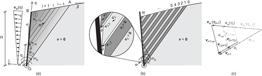
Kinematically admissible failure mechanism caused by a rotation of the wall about the point O: (a) boundary conditions and velocity of an infinitesimal slice; (b) graphical representation of the velocity field; (c) velocity diagram for three adjacent infinitesimal slices. The infinitesimal slices are depicted with a finite thickness solely for illustrative purposes
Kinematically admissible failure mechanism caused by a rotation of the wall about the point O: (a) boundary conditions and velocity of an infinitesimal slice; (b) graphical representation of the velocity field; (c) velocity diagram for three adjacent infinitesimal slices. The infinitesimal slices are depicted with a finite thickness solely for illustrative purposes
Assuming that the wall undergoes a virtual rotation increment ω about point O, either due to the formation of a plastic hinge or lack of sufficient support, it results in the displacement of the wall with a virtual velocity vw(η) = ωη perpendicular to it. This displacement causes the soil to deform and unload, leading to active failure in the limit state. While translational wall displacement results in a single slip line, rotational displacement requires the formation of a shear zone that undergoes a continuum deformation to satisfy the kinematic boundary conditions, as illustrated in Figs 2(a) and 2(b). An idealised representation of the continuum shear zone comprises an infinite number of rigid slices, each with infinitesimal thickness, that move virtually to follow the wall rotation obeying the associated flow rule. In this context, the associated flow rule prescribes that each slice of soil moves away from the slice below it with a velocity increment inclined by an angle equivalent to the soil friction angle (i.e. ψ ≡ ϕ). Fig. 2(a) shows three of these slices with finite thickness for illustrative purposes. The relative velocity v(i−1),i at the discontinuity between slice i and slice (i − 1) and the relative velocity vi,w between slice i and the wall are shown. The associated flow rule causes slice i to move away from slice (i − 1) at a relative velocity inclined by an angle ϕ with respect to the slip line, as shown in Fig. 2(b). Although frictional interfaces are generally non-dilatant (i.e. ψ = 0), the velocity at the soil–wall interface can be assumed to have an inclination defined by the interface friction angle δ according to Drucker's friction theorem C (Drucker, 1954). As a result, the rate of dissipation at the interface becomes zero.
The failing soil wedge is supported on the left by the wall and on the right by a rigid block of soil (block 0 in Fig. 2(b)) at rest (i.e. v0 = 0). In the shear zone, the virtual velocity field is variable, as represented in Fig. 2(a) by a greyscale gradient. Slice 1 remains stationary since the wall impedes its movement
Therefore, the velocity of slice 2 can be calculated as
This implies that the velocity of slice 2 aligns with the direction of the relative velocity v1,2, which has an inclination angle of ϕ to the slip line. To comply with the flow rule, slice 3 must have the same velocity direction. In fact, its velocity is given by
Given that velocities v2 and v2,3 have the same direction (as seen in Fig. 2(b)), it is evident that v3 must be parallel to them. This leads to a self-similar velocity diagram for all slices in the OAB shear zone, which is illustrated in Fig. 2(c) for three adjacent slices. Hence, the velocity field of the entire shear zone can be completely described in terms of the Cartesian coordinate η describing their position along the soil–wall interface (i.e. at ξ = 0)
The velocity of a soil slice is denoted by vs(η) and the velocity of the wall is represented by vw(η). The velocity diagram defines the matrix C, which remains unchanged over the entire shear zone.
The limit load ma can be calculated by equating the combined rate of external work performed by the weight of the slices, , and by the resisting moment ma, , to the rate of dissipation
Because a purely frictional soil is assumed (i.e. c = 0) and because of the adoption of Drucker's friction theorem C (Drucker, 1954), the dissipation rate is zero
While the solution of the mechanism in Fig. 2 provides a simple application in practice, a more accurate calculation of the ultimate load can be obtained by considering more complex mechanisms, such as those shown in Fig. 3, which involve a combination of shear zones separated by velocity discontinuities. In Fig. 3, the variable velocity field is represented by a greyscale gradient. In contrast, the velocity vectors drawn along the discontinuity lines only indicate the direction of this velocity, which is the same within each triangular region bounded by discontinuity lines.
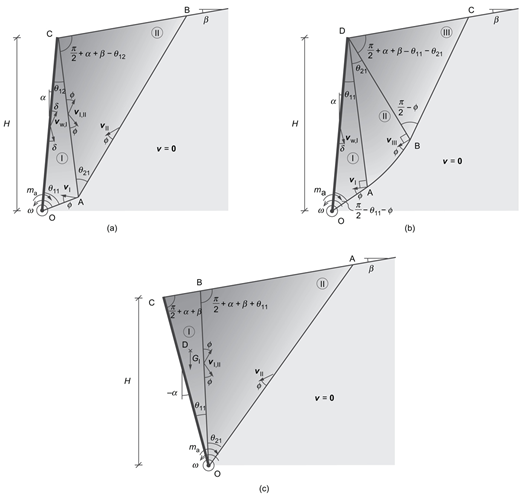
Failure mechanisms: (a) two wedges; (b) wedge–logarithmic spiral–wedge; (c) extended single wedge. The greyscale gradient qualitatively represents the magnitude of the velocity of a material point
Failure mechanisms: (a) two wedges; (b) wedge–logarithmic spiral–wedge; (c) extended single wedge. The greyscale gradient qualitatively represents the magnitude of the velocity of a material point
In frictional materials, only linear and logarithmic spiral-shaped slip lines are kinematically admissible, as outlined by Chen (1975). With this in mind, two different types of shear zones, a wedge and a logarithmic spiral sector, both undergoing homogeneous shear deformation, are analysed in the following sections.
First, the rate of external work done by the soil for each of these two types of shear zones is formulated in a generally applicable manner, assuming a variable velocity field. These elements can then be appropriately combined to solve the earth pressure problem considered in this article.
It is worth noting that while Chen (1975) dealt with homogeneous shear deformation in a weightless, cohesive soil, there remains a gap in the literature for a more thorough formulation that considers a frictional soil of finite weight. Therefore, the proposed general formulation could be a valuable tool for developing solutions to various geotechnical problems, especially those involving rotation.
Wedge-shaped shear zone
Consider the triangle OAB depicted in Fig. 4 composed of soil with friction angle ϕ and unit weight γ, which is subjected to a virtual velocity field entirely described by the linear function vs(η) along the edge. The wedge can be divided into infinitesimal slices of thickness dh and finite length l(η) such as the one drawn in dark grey in Fig. 4 and inclined by θ4 to the horizontal. Here, the slices are assumed to be parallel to the edge . The virtual velocity of each slice is expressed by the linear function
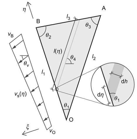
Wedge-shaped shear zone subjected to a variable velocity field
Wedge-shaped shear zone subjected to a variable velocity field
The velocity vector is inclined to the horizontal by the angle θv. The angle is restricted by the equation θ4 − θv = ϕ to achieve a self-similar velocity diagram as in Fig. 2(c).
Considering the geometrical parameters l1, θ1, θ2 to be known (they are related to the remaining lengths and angle through the law of sines), the infinitesimal area of a slice reads
Therefore, the external work rate done by the soil in the wedge can be written as
Logarithmic spiral sector shear zone
Consider the logarithmic spiral sector in Fig. 5 composed of soil with friction angle ϕ and unit weight γ, which is subject to a virtual velocity field described entirely by the linear function vs(r, χ = 0) along the edge
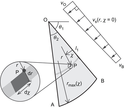
Shear zone defined as a logarithmic spiral sector and subjected to a variable velocity field
Shear zone defined as a logarithmic spiral sector and subjected to a variable velocity field
Owing to the properties of the logarithmic spiral, defined by the polar equation r = aexp(bχ), the virtual velocity of an arbitrary material point located in the sector OAB can be expressed as
The direction of the velocity vector in a logarithmic spiral sector is perpendicular to the position vector . The logarithmic spiral sector can be ideally divided into infinitesimal surface elements of an area
each virtually displacing with velocity vs(r, χ) by satisfying the associated flow rule and the prescribed conditions.
Thus, the external work rate done by the soil can be expressed as
with
Integrating equation (14), one obtains
Active earth pressure acting on walls subject to rotation about the wall base: single wedge mechanism
The moment exerted on the wall in Fig. 2 in the limit state can be determined using equations (6) and (10). Two possible velocity diagrams, shown in Figs 6(a) and 6(b), describe the kinematics of the problem, depending on the direction of the relative velocity at the soil–wall interface (either pointing upwards or downwards). The magnitude of the virtual velocity of a soil slice in the shear zone OAB (otherwise defined as wedge I) reads

Velocity diagrams for the mechanisms depicted in Figs 2 and 3: (a), (b) kinematics of a wedge-shaped shear zone that is in contact with a body undergoing rigid-body motion, such as a wall or soil rigid block; (c), (d) kinematics of wedge 2 in the two-wedges mechanism in Fig. 3(a); (e) kinematics of the logarithmic spiral sector in the mechanism depicted in Fig. 3(b)
Velocity diagrams for the mechanisms depicted in Figs 2 and 3: (a), (b) kinematics of a wedge-shaped shear zone that is in contact with a body undergoing rigid-body motion, such as a wall or soil rigid block; (c), (d) kinematics of wedge 2 in the two-wedges mechanism in Fig. 3(a); (e) kinematics of the logarithmic spiral sector in the mechanism depicted in Fig. 3(b)
At a specific point, the tangential velocity of the wall is expressed as
The angle between the velocity vector and the horizontal is
The rate of work generated by the resisting moment ma reads
As mentioned previously, with dissipation being zero, the virtual work equation reads
The rate of energy was given in equation (10). The moment ma exerted on the wall when active soil failure occurs can be expressed as a function of the free parameter θ11
Solving the following constrained optimisation problem provides the most critical failure mechanism
Active earth pressure acting on walls subject to rotation about the wall base: improved mechanisms
Considering the mechanisms illustrated in Fig. 3 can lead to an improved solution. The two mechanisms depicted in Figs 3(a) and 3(b) were introduced for a translational wall displacement by Chen (1975) and are re-evaluated in this study by introducing a rotational wall motion. The mechanism shown in Fig. 3(a) consists of two wedges separated by a velocity discontinuity and is fully characterised by three parameters θ11, θ12 and θ21. Wedge I has the same kinematics as the single wedge mechanism and is characterised by the velocity diagrams in Figs 6(a) and 6(b). The magnitude of the virtual velocity of a soil slice in that wedge is therefore described by equation (17). Similarly to wedge I, two velocity diagrams are possible for wedge II (Figs 6(c) and 6(d)), depending on the direction of the relative velocity along the discontinuity line (either pointing upwards or downwards). The virtual velocity magnitude of the soil undergoes a linear increase between points A and C due to the shearing deformation of wedge I. It starts from zero and reaches the following maximum value at point C
These two cases correspond to the diagrams shown in Figs 6(c) and 6(d). In wedge II, the angle between the horizontal and the virtual velocity vector is determined as follows
The rate of external energy done by the two wedges is formulated according to equation (10)
Combining equations (6), (7), (20) and (26), the moment ma exerted on the wall when active soil failure occurs can be expressed as a function of the free parameters θ11, θ12 and θ21
This equation is subject to many constraints, which can be divided into two categories: general constraints and specific constraints for each configuration of the velocity diagrams. The general constraints must be satisfied by each possible configuration of the mechanism and are as follows
The specific constraints for each velocity diagram are designed to ensure the validity of the angles in a specific configuration of the velocity diagram (Figs 6(a)–6(d)) – that is the angles formed by the velocity vectors must satisfy 0 < θij < π. For readers interested in the detailed formulation of these constraints, the complete code implementing the constraints and the associated limit analysis is shared according to the code sharing statement at the end of this paper.
In a similar way to the single wedge mechanism, the most critical failure mechanism is found by solving a constrained optimisation problem.
The mechanism in Fig. 3(b) consists of two wedges separated by a shear zone defined by a logarithmic spiral and is fully characterised by two parameters, namely θ11 and θ21. Assuming the slip line OABC to be continuously differentiable, the remaining angles result from the problem geometry and the properties of the logarithmic spiral. In addition, no sliding occurs along and (i.e. the relative velocity is zero). The velocity diagram in Fig. 6(a) describes the kinematics of wedge I. In this case, the relative velocity at the soil–wall interface always points downwards because when the velocity vI would be equivalent to the wall velocity vw, vI ≡ vw in the corner case θ12 = 0. It follows that
with vw(η) defined as in equation (18).
The kinematics of blocks II and III is described by Fig. 6(e). In the logarithmic shear zone, the magnitude of the virtual velocity decreases, so that at point D in wedge III it reads
The direction of the virtual velocity vector (with respect to the horizontal) in wedge I is
In the logarithmic spiral, the direction is variable, while in wedge III it is
Furthermore, the length of the segment can be written as
The rate of external energy done by the two wedges and the logarithmic spiral sector is formulated according to equations (10) and (16)
Combining equations (6), (7), (20) and (34), the moment ma exerted on the wall when active soil failure occurs can be expressed as a function of the free parameters θ11 and θ21
The most critical failure mechanism is found by solving an optimisation problem subject to the following constraints
Figure 3(c) represents an extension of the single wedge mechanism illustrated in Fig. 2. It considers the rigid body rotation of wedge I around point O, which follows the rotation of the wall, and the shearing of wedge II.
The kinematics of wedge I is the same as that of the wall – that is a rigid body rotation about point O with angular velocity ω. The position of the centroid of wedge I (point D in Fig. 3(c)) is given by the arithmetic mean of the coordinates of its vertices
The length of the discontinuity line between wedges I and II is
The weight of wedge I can therefore be written as
The virtual velocity at the centroid of wedge I can be expressed as
The rate of external work done by wedge I can therefore be calculated as the scalar product of the virtual velocity and the weight vector GI (a vertical vector having magnitude GI)
Wedge II, instead, exhibits the same kinematics as the wedge in the single wedge mechanism shown in Fig. 2, except for the friction angle at the velocity discontinuity , which is equal to the soil friction angle in this case. Hence, considering δ: = ϕ, the kinematics of wedge I is described by Figs 6(a) and 6(b). The total moment acting at point O is therefore given by:
where
The most critical failure mechanism is found by solving an optimisation problem subject to the following constraints
APPROXIMATE STATIC SOLUTION: EXTENDED LANCELLOTTA'S SOLUTION
A static solution for the active earth pressure acting on a vertical wall was proposed by Lancellotta (2002). This solution was later extended by Perozzi (2022) to account for walls and soil with arbitrary inclinations. Consider a wall with height H and inclined at an angle α to the vertical. The wall supports a granular backfill having a surface inclination β and shear strength characterised by the angle of internal friction ϕ. According to this solution, the moment that acts on the wall at its base in the active state can be written as (Perozzi, 2022)
where
While this solution was originally suggested by Lancellotta (2002) as a rigorous bound of the exact solution, and was also presented as such by Perozzi (2022), it does exhibit partial violations of the equilibrium equations near the wall and is not a strict bound. Nonetheless, the solution obtained is always observed to be more conservative than the kinematic one (Perozzi, 2022).
RESULTS AND DISCUSSION
Following the conventional practice in earth pressure problems, a load coefficient (see, e.g. Nadukuru & Michalowski (2012) and Perozzi (2022)) is introduced as a normalised measure of the moment acting at the wall base
It is essential to note that this coefficient does not relate in any way to a stress distribution.
In this section, only the load coefficient (instead of the absolute value of the moment) is used to study the ultimate load on walls rotating around the base. When plotting the load coefficient resulting from the proposed kinematic solution, all the mechanisms shown in Figs 2 and 3 are considered to identify the most critical one for each parameter set, and only the highest value is presented in the plot. Interestingly, for none of the parameter sets considered does the mechanism shown in Fig. 3(b) prove to be the most critical. This suggests that the assumption of a logarithmic spiral centred at the top of the wall may be too restrictive.
Kinematic solution, extended Lancellotta and numerical solution
Figure 7 compares the developed kinematic solution, Lancellotta's extended solution and a finite-element-based limit analysis (FELA) solution obtained using the Optum G2 software with adaptive remeshing (Optum Computational Engineering, 2021). The kinematic and static solutions from Optum are very close. Thus, the slightly more conservative static solution is chosen for consideration. Three wall inclinations and a variable backfill inclination are examined, assuming a soil friction angle of 30° and a wall friction angle of 20°. In general, the kinematic solution and the improved Lancellotta's solution permit an accurate estimate of the exact solution, which is nearly equivalent to Optum's solution. Although the approximated static solution may become excessively conservative for positive wall inclinations, it still provides a reliable and conservative estimation of the limit load under the most frequently encountered conditions. Moreover, its straightforward closed-form solution makes it user-friendly and easy to apply. Numerical values for the kinematic solution developed are given in the Appendix and can also be calculated using the code provided with this paper.
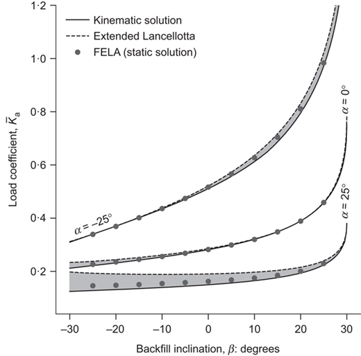
Comparison of load coefficients derived from three different solutions: kinematic solution, extended Lancellotta's solution, and the FELA-based solution. A wall with different inclinations α and variable backfill inclination β is considered. The soil friction angle is ϕ = 30°, and the wall friction angle δ = 20°
Comparison of load coefficients derived from three different solutions: kinematic solution, extended Lancellotta's solution, and the FELA-based solution. A wall with different inclinations α and variable backfill inclination β is considered. The soil friction angle is ϕ = 30°, and the wall friction angle δ = 20°
Assessment of traditional design methods
Although the limit load behind rotating walls has been widely discussed in the literature, a significant gap remains: no practical method has been established or developed, and earth pressure calculations typically rely on the assumption of translational wall displacement, using solutions such as the Coulomb method and assuming an arbitrary linear stress distribution. Specifically, the following equation is frequently used to calculate the moment acting on the wall
Here, ean represents the perpendicular component of total earth pressure on the wall.
To evaluate common design methods and explore possible peculiarities of the limit load acting on rotating walls, the following analysis is carried out. First, the load coefficients determined using the proposed kinematic solution are presented in Fig. 8, denoted ‘ROT’ (rotation about the base). It is plotted as a function of the backfill inclination β for different values of soil friction angle ϕ and wall inclination α. The calculation always assumes a wall interface friction of δ = 2/3 ϕ. Then, the load factor is calculated using equation (50). The earth pressure ean is calculated considering the same type of mechanisms as in Figs 2 and 3, with the wall undergoing a horizontal translation instead of a rotation. The obtained values are plotted in Fig. 8 and labelled ‘T’ (translation).
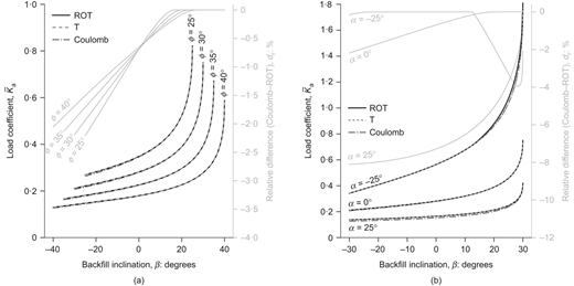
Comparison of load coefficients derived from three different approaches: using the proposed kinematic solution assuming a rotating wall (ROT), assuming the earth pressure from a wall translating horizontally acting at one-third of the wall height (T), and assuming Coulomb's earth pressure acting at one-third of the wall height (Coulomb). (a) Assuming α = 0° and δ = 2/3ϕ; (b) assuming ϕ = 30° and δ = 20°
Comparison of load coefficients derived from three different approaches: using the proposed kinematic solution assuming a rotating wall (ROT), assuming the earth pressure from a wall translating horizontally acting at one-third of the wall height (T), and assuming Coulomb's earth pressure acting at one-third of the wall height (Coulomb). (a) Assuming α = 0° and δ = 2/3ϕ; (b) assuming ϕ = 30° and δ = 20°
Considering a vertical wall (Fig. 8(a)), it is clear that the load factor calculated assuming wall translation as in equation (50) is identical to that resulting from wall rotation. This equivalence results from the similar velocity diagram of an infinitesimal soil slice. In fact, the virtual velocity of the wall remains horizontal in both scenarios (the tangential velocity of a rotating vertical wall is horizontal). Similar observations can be made when considering a positive wall inclination (e.g. α = 25° in Fig. 8(b)), but not for a negative wall inclination (e.g. α = −25° in Fig. 8(b)). In the case of a positive inclination, the relative velocity at the soil–wall interface points in the same direction (i.e. downwards), regardless of whether rotation or translation is considered. This gives the velocity diagram shown in Fig. 6(a) and results in the same limit load. However, in the case of a negative wall inclination, for example α = −25°, it may be that the most critical failure mechanism differs from that of a translational failure mode. This is the case, for example, in Fig. 8(b) for β = 25°. In this configuration, the single wedge mechanism governs the translational failure mode (Fig. 9(a)). Considering the same critical configuration (i.e. the same inclination of the failure line) of the single wedge mechanism for the rotational wall displacement would lead to the velocity diagram in Fig. 6(b) – that is, with the relative velocity at the interface pointing upwards. However, this configuration is less favourable in energetic terms, so the inclination of the failure line remains constrained by θ11 ≤ π/2 − ϕ, as observed in Fig. 9(a). In general, therefore, it can be said that the same load coefficient results from the translational and rotational single wedge failure mechanisms only if the optimised configuration of the translational mechanism satisfies the relation θT11, crit ≤ π/2 − ϕ. As this relation is not satisfied for the case α = −25° and β = 25°, the extended single wedge mechanism becomes governing for the rotation about the bottom (Fig. 9(b)), leading to a higher load coefficient than that estimated assuming a translation.
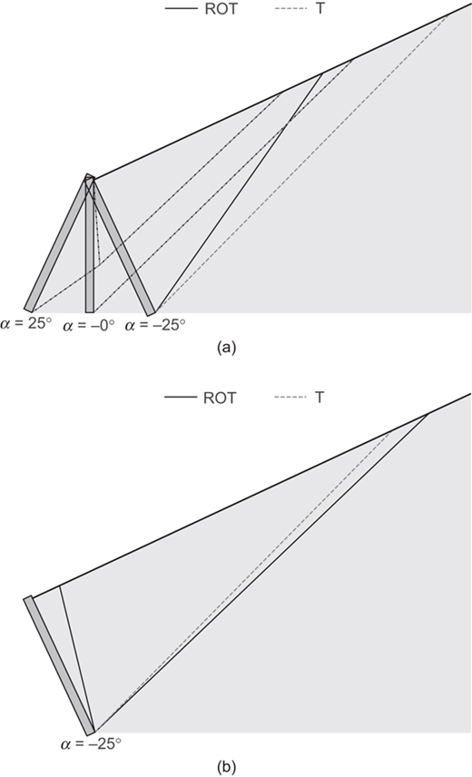
Optimised failure mechanisms for parameters β = 25°, δ = 20° and ϕ = 30° and two distinct displacement modes: translation (T) and rotation about the base (ROT). In (a), different wall inclinations and the failure mechanisms in Figs 2, 3(a) and 3(b) are considered. In (b), only a wall inclined by α = −25° and all failure mechanisms in Figs 2 and 3 are considered
Optimised failure mechanisms for parameters β = 25°, δ = 20° and ϕ = 30° and two distinct displacement modes: translation (T) and rotation about the base (ROT). In (a), different wall inclinations and the failure mechanisms in Figs 2, 3(a) and 3(b) are considered. In (b), only a wall inclined by α = −25° and all failure mechanisms in Figs 2 and 3 are considered
In addition, Fig. 8 shows the load coefficient obtained by applying equations (49) and (50) using Coulomb's total earth pressure. It can be seen that this solution provides a reasonably accurate estimate for vertical walls and for walls with a negative inclination. However, special attention is required when dealing with walls inclined positively. In such cases, Coulomb's assumption of a linear failure line leads to an underestimation of the ultimate load of up to 8% compared to the proposed kinematic solution. This discrepancy arises because an inclined wall induces a more significant rotation of the stress state near the wall, which can be better captured by considering additional velocity discontinuities.
In general, it can be said that common practice gives a reasonably accurate estimate of the limit load for the most common parameters.
Experimental validation
The experimental data collected by Fang & Ishibashi (1986) are a standard reference in the literature for validating analytical models that predict earth pressure on walls experiencing various displacement modes. While several authors in the past focused mainly on the earth pressure distribution measured at the rotation of 1·5 mrad (reported in their figure 12), assuming that the active state had already been reached, it is interesting to look at figure 13 in their publication. In the figure it can be seen that at the rotation of 1·5 mrad only the mobilised wall friction has already reached a steady value, while both the horizontal earth pressure and its location are still changing, indicating that the ultimate state has not yet been reached. In fact, the active state seems to be reached only after a rotation of 6 mrad. Therefore, to validate a limit state solution properly, only the data from the second graph should be considered. The wall in Fang & Ishibashi's (1986) experiment had to resist a moment given by
Here, KFIh is Fang and Ishibashi's measured load coefficient, and h is the measured point of application (measured from the wall base). This can be reduced to the load factor as in equation (49)
For a loose sample, they measured KFIh ≈ 0·26 and h/H ≈ 0·281, which leads to . The soil friction and wall friction angles are ϕ = 33·4° and δ = 23·8°, respectively. The experimental result and the value predicted by the proposed solution are summarised in Table 1.
Comparison of predicted load coefficient (kinematic solution) and experimental data
| Author(s) | Soil density | Load coefficient, | |
|---|---|---|---|
| Experiment | Kinematic solution | ||
| Fang & Ishibashi (1986) | Loose | 0·22 | 0·24 |
| Perozzi (2022) | Loose | 0·20 | 0·21 |
| Dense (peak) | 0·10 | 0·10 | |
| Dense (residual) | 0·15 | 0·21 | |
Recently, Perozzi (2022) conducted an experimental parametric study on the earth pressure acting on a wall rotating about the base. A retaining wall was backfilled with either loose (10% relative density) or dense (95% relative density) soil and a rotation of up to 35 mrad was induced at its base. Dry uniform silica sand was used. The residual and peak friction angles measured under plane-strain conditions are 37° and 52°, respectively. The measured wall friction angle was determined to be 22° for both soil densities. The moment exerted by the dense backfill on the wall first reached a minimum value characterised by the load coefficient when peak strength is mobilised. Owing to softening of the soil, the load coefficient subsequently increased to . In contrast, for the loose sample, the load coefficient progressively decreased as the wall rotation increased. The relevant experimental and analytical results are summarised in Table 1.
It is observed that the analytical values align closely with the experimental results, except for the residual value measured in the dense sample by Perozzi (2022). In that particular case, the analytical solution gives a value 40% higher than the experimental result. This is mainly due to soil softening, leading to strain localisation and a non-linear earth pressure distribution. This complex behaviour, known to cause a non-unique soil mechanical response (Rice, 1976; Bigoni & Hueckel, 1991), cannot be accurately represented through analytical methods (and special care is needed when using finite-element-based elastoplastic calculations). Hence, designers shall rely on conservative solutions based on perfect plasticity and assume the residual value of soil friction.
Furthermore, it can be noted that, although the kinematic solution should provide a lower bound for the exact solution according to equation (1), the experimental results are consistently lower than the value predicted by the kinematic solution. This is due, at least partly, to the fact that limit analysis only considers undeformed configurations, whereas in reality the point of application of the resultant force is continuously lowered as a result of the wall rotation and soil deformation (Perozzi, 2022).
CONCLUSIONS
The design and verification of geotechnical structures require accurate determination of the forces and moments induced by the earth pressure in the active failure state. Traditional methods for calculating active earth pressure do not provide reliable information on the pressure distribution, which is often assumed to be linear, although previous studies have shown that this distribution depends on the mode of wall displacement. However, in ultimate state design, the stress distribution is not required, as only the internal force associated with the relevant failure mode, such as rotation in the case of bending failure, is required. Therefore, solutions based on limit analysis are well suited for the design and verification of retaining structures.
This paper has investigated the limit load on a wall rotating about its base. First, a rigorous kinematic solution was analytically formulated. This solution is the first of its kind in that it considers the homogeneous shear deformation over a soil region possessing finite weight. This solution was then compared to an approximate static solution and to a FELA solution. Based on these solutions, it is possible to bracket the ultimate load efficiently. While the kinematic solution is closer to the FELA solution (but lies on the unconservative side), the approximate static solution provides a reasonable, conservative estimate for common parameters, and is available in a closed form, which facilitates its use in practice.
Subsequently, it was observed that calculating the ultimate moment assuming the force derived from a translational mechanism applied at one-third of the wall height delivers the same result as the proposed, more rigorous kinematic solution for the most common soil parameters and geometries. Therefore, traditional designs where a Coulomb's resultant force was applied at one-third of the height to calculate ultimate moments are reasonably safe.
Finally, the proposed limit analysis solution was successfully validated using both the existing and new experimental data, confirming its effectiveness in providing a safe solution. Furthermore, this validation indirectly supports the traditional design methods used in practice. It should be noted that in the case of a dense soil, a non-linear pressure distribution becomes a significant factor at the residual state. However, accurately capturing this behaviour is a challenge for analytical tools due to the highly complex and non-linear nature of soil behaviour. Consequently, engineers are forced to rely on the conservative assumption of perfect plasticity using the residual value of the friction angle.
The solution presented here eliminates the need to quantify the earth pressure distribution in the ultimate limit state using semi-empirical approaches. While other design tasks, such as deflection control, may still require knowledge of the pressure distribution, they represent serviceability limit states and should not assume active soil failure to occur everywhere in the backfill. Instead, an elastoplastic analysis becomes necessary.
Code availability statement
The software code associated with this research has been archived and is available by way of the following digital object identifier: https://doi.org/10.3929/ethz-b-000634100.
For the latest version, ongoing development, or to contribute, the code can also be accessed on GitHub at: https://github.com/dperozzi/active-earth-pressure.
ACKNOWLEDGEMENTS
The authors thank Dr Balz Friedli, Dr Dominik Hauswirth, Roman Hettelingh, Boaz Klein and Marc Kohler (all ETH Zurich, Switzerland) for their valuable input and discussions. The work was supported by the Swiss Federal Roads Office and the Swiss Federal Office of Transport (research project AGB 2015/029).
NOTATION
- A
area of a soil region
- c
soil cohesion
rate of internal dissipation
- ean
total active earth pressure acting perpendicular to the wall
- H
wall height
- h
vertical distance from base to point of applied horizontal earth pressure, observed in Fang & Ishibashi (1986)
- Kan
active earth pressure coefficient related to the stresses along the wall in perpendicular direction
load coefficient – that is, a normalised measure of the moment on the wall
- KFIh
coefficient of horizontal earth pressure, as measured in Fang & Ishibashi (1986)
- li
length of segment i
- ma
moment exerted on the wall by the active earth pressure (by extension, resisting moment needed to prevent active failure)
- r, χ
system of polar coordinates
- v
vector
- v
vector v's magnitude
- vI
virtual velocity of soil in velocity region denoted by the Roman numeral I
- vi
virtual velocity of the ith infinitesimal slice
- vi,j
virtual relative velocity at the interface between bodies i and j
- vw, vs
virtual velocity of the wall and the soil, respectively
rate of external work done by the resisting moment and by the soil weight, respectively
- α
wall inclination
- β
backfill inclination
- γ
soil unit weight
- δ
wall friction angle
- η, ξ
Cartesian coordinate system
- θij
parameter defining the size of the angles of a velocity region
- θv
inclination of the velocity increment
- μ, ζ
parameters of the extended Lancellotta solution
- ϕ
soil friction angle
- ψ
soil dilatancy angle
- ω
virtual rotation increment
REFERENCES
APPENDIX: EARTH PRESSURE TABLE
The active earth pressure coefficients given in Table 2 are calculated according to its definition in equation (49) based on the kinematic solution presented in this paper. These coefficients are calculated for different friction angles ϕ and different wall and backfill inclinations. The table is generated considering all the failure mechanisms discussed in this paper and illustrated in Figs 2 and 3. The friction angle at the soil–wall interface is consistently kept at δ = 2/3ϕ. For values corresponding to other parameters or scenarios, the reader can refer to the code accompanying this article.
Active earth pressure coefficients
| Soil friction angle, ϕ: degrees | Backfill inclination, β: degrees | Wall inclination, α: degrees | ||||
|---|---|---|---|---|---|---|
| −20 | −10 | 0 | 10 | 20 | ||
| 25 | −10 | 0·4429 | 0·3693 | 0·3110 | 0·2622 | 0·2184 |
| 0 | 0·5175 | 0·4212 | 0·3480 | 0·2893 | 0·2383 | |
| 10 | 0·6239 | 0·4982 | 0·4040 | 0·3309 | 0·2696 | |
| 20 | 0·8424 | 0·6531 | 0·5226 | 0·4216 | 0·3399 | |
| 30 | −10 | 0·3888 | 0·3132 | 0·2538 | 0·2043 | 0·1603 |
| 0 | 0·4505 | 0·3542 | 0·2813 | 0·2231 | 0·1730 | |
| 10 | 0·5334 | 0·4112 | 0·3203 | 0·2502 | 0·1916 | |
| 20 | 0·6722 | 0·5077 | 0·3892 | 0·2989 | 0·2261 | |
| 30 | 1·3996 | 1·0217 | 0·7500 | 0·5773 | 0·4398 | |
| 35 | −10 | 0·3411 | 0·2648 | 0·2057 | 0·1574 | 0·1151 |
| 0 | 0·3918 | 0·2970 | 0·2260 | 0·1701 | 0·1229 | |
| 10 | 0·4569 | 0·3394 | 0·2531 | 0·1875 | 0·1338 | |
| 20 | 0·5550 | 0·4042 | 0·2962 | 0·2157 | 0·1518 | |
| 30 | 0·7876 | 0·5446 | 0·3938 | 0·2818 | 0·1957 | |
| 40 | −10 | 0·2987 | 0·2229 | 0·1652 | 0·1191 | 0·0801 |
| 0 | 0·3401 | 0·2479 | 0·1798 | 0·1276 | 0·0846 | |
| 10 | 0·3913 | 0·2792 | 0·1985 | 0·1385 | 0·0907 | |
| 20 | 0·4633 | 0·3241 | 0·2261 | 0·1550 | 0·1000 | |
| 30 | 0·6051 | 0·4042 | 0·2776 | 0·1865 | 0·1184 | |
| 40 | 1·3892 | 0·9094 | 0·5868 | 0·3974 | 0·2554 | |
Discussion on this paper closes 1 May 2026; for further details see p. ii.

