


This paper presents a new formulation of the problem of tunnelling effects on pipelines, which incorporates the tunnel kinematic constraints in the tunnel–soil–pipeline interaction analysis. This ‘constrained continuum formulation’ can be considered an extension of the original ‘two-stage’ elastic-continuum method, which traditionally neglects the mutual influence of the pipeline on the tunnel and vice versa. The new approach retains the advantage of using the greenfield condition as an input, but it allows closed-form consideration of the stiffening effect of the tunnel on the soil domain. The paper details the formulation and then provides an investigation into the effect of varying fixities: namely, both as ‘wished-in-place’ tunnels and as evolving, advancing constraints, with the tunnel ‘construction’. Normalised solutions are presented and compared with the previous formulation. In general, the addition of tunnel constraints leads to a stiffer soil action, and thus higher bending stressing in the pipeline; modelling of the tunnel kinematic constraint is conservative. The question of when such analysis is desired is discussed, concluding with a simple-to-use inequality suitable for design.
INTRODUCTION
The underground space in a modern city contains intricate systems of tunnels, pipelines and various forms of buried infrastructure. As such, new infrastructure development must account for the effect of the new construction on existing nearby buried tunnels and pipelines. The assessment of tunnelling effects on existing buried pipelines has been addressed by researchers over the last 20 years, who have proposed engineering tools to predict the distress induced in the existing infrastructure (e.g. Vorster et al., 2005; Klar & Marshall, 2008; Marshall et al., 2010; Wang et al., 2011; Yu et al., 2013; Wham et al., 2016; Ieronymaki & Whittle, 2017; Zhang et al., 2019; Klar, 2022).
One of the central approaches developed over the years is the matrix-based elastic continuum formulation of Klar et al. (2005). This approach has been widely adopted, and was even extended to other cases including soil non-linearity (Klar et al., 2007, 2016), jointed pipelines (Klar et al., 2008), layered soil (Zhang & Huang, 2012) and Timoshenko beam theory (Franza & Viggiani, 2021). Furthermore, it has been validated by more refined solutions, based on Fourier analysis, in which full cross-sectional as well as longitudinal compatibility are enforced (Klar, 2018, 2022; Klar & Shoham, 2022).
It has also been adopted over the years for the treatment of the ‘sister’ problems of tunnelling effects on buildings and piles (e.g. Elkayam & Klar, 2019; Franza & DeJong, 2019; Franza et al., 2020a, 2021a, 2021b).
There were several assumptions involved in the linear elastic continuum solution of Klar et al. (2005): (a) that the pipeline is always in contact with the soil; (b) that the soil is homogeneous; (c) that the pipeline does not affect the tunnel; (d) that the soil response at the pipeline level is not aware of the tunnel; (e) that the pipeline is continuous; and (f) that the greenfield settlements are represented by a Gaussian function. Assumption (a) is inherent to linear elastic formulations, and simply infers that no gaps develop between the pipeline and the soil irrespective of the magnitude of the greenfield displacement field, leading the solution to be linearly dependent on the magnitude of the greenfield displacement. Assumptions (b), (e) and (f) are not central to the solution, as a different greenfield input, and soil and pipeline conditions, could be considered without substantial modification of the matrix-based formulation, as for previous works.
Assumptions (c) and (d), however, are central to the formulation, allowing for direct use of the greenfield input. In fact, the use of the greenfield input has led to the use of the term ‘two-stage’ method for this approach, to emphasise that the process is decoupled. In other words, the original formulation deals with the soil–pipeline interaction resulting from the tunnelling-induced ground deformation, and it does not involve any mechanical action of the tunnel in the interaction analysis.
The proposed formulation in the paper avoids assumptions (c) and (d), and instead introduces the kinematic constraints caused by the tunnel as a restraint of the continuum vertical movement at the excavation periphery, with an effect on the soil–pipeline interaction. Fig. 1 illustrates this concept, in which a new tunnel is being excavated below an existing pipeline. In the classical ‘two-stage’ method, the induced ground deformation is translated to external forces acting on the pipeline, which deforms based on the soil–pipe interaction. In the current formulation, additional constraints are added to the elastic continuum that prevent tunnel deformations due to the pipeline response, leading the solution to truly involve tunnel–soil–pipeline interaction (due to the interaction between the pipeline and the kinematic constraint).
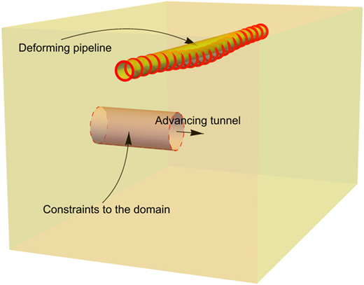
Illustration of the problem and the additional constraints
Illustration of the problem and the additional constraints
The paper is composed of four main sections. First, the adoption of the tunnel kinematic constraints to the continuum interaction model is detailed. Then, this new formulation is compared to the classical ‘two-stage’ approach. Next, an engineering discussion is presented, dealing with whether and when the constrained continuum analysis is desired. Finally, conclusions are drawn.
FORMULATION
The original formulation
In the original formulation of Klar et al. (2005) the displacement of the soil continuum, uC, was decomposed into a local displacement uCL (due to loading at the considered point) and an additional displacement uCA (due to loading at any other locations). The additional continuum displacement uCA was further decomposed into that generated by forces exerted by the pipeline uCAP and that originated from the tunnel uCAT. Under the assumption that the tunnel is not affected by the pipeline uCAT was replaced by ugf. In Klar et al. (2005) the relations between forces acting on the soil and the displacement are presented using matrices to represent the summation process of all contributors:
and in matrix form as
where K* and λ*s are given by
where Gi,j is the Green's function that defines the elastic continuum displacement at point i due to loading at point j. For homogeneous half-space, the solution by Mindlin (1936) can be used to construct Gi,j.
The pipeline behaviour itself (as an isolated structure) can be represented using a stiffness matrix:
where S is the stiffness matrix of the pipeline and F denotes the forces acting on the pipeline. Compatibility requirements between the pipeline and the soil lead u to be equal to uC, and equilibrium requirements f = −F = −Su. Multiplying equation (2) by K* and substituting − Su for f results in the following expression:
All matrices involved in this formulation are square, n × n, where n is the number of pipeline degrees of freedom. For the sake of simplicity, soil–pipeline interaction is considered to occur only in the vertical degrees of freedom.
Note that the use of ugf for uCAT infers that the interaction forces between the tunnel and the soil are not changed due to the existence of the pipeline. As such, one may claim that the original solution actually corresponds to an ‘infinitely flexible’ tunnel (as the flexible tunnel is unable to change the forces acting on the soil).
This is mentioned because the alternative formulation, presented in the subsequent subsection, is based on the other extreme condition of an ‘infinitely stiff’ tunnel, where there are additional kinematic constraints in the soil domain that prevent movement.
The new constrained continuum formulation
The stiffening action of the tunnel lining is treated in this paper as a fixed constraint in space. That is, the ‘constructed’ tunnel is assumed to be vertically fixed and does not deform due to the soil–pipe interaction. This is an extreme condition, as tunnels have finite stiffness and, therefore, may deform due to the response of the pipeline both longitudinally and within the cross-section. While the original formulation assumed an ‘infinitely flexible’ tunnel, the current one assumes an ‘infinitely stiff’ tunnel with a constrained continuum. These two solutions should in principle bracket any realistic condition in which the tunnel has a finite stiffness.
The notion of immobility of the tunnel is a mathematical assumption that schematises a complex boring machine–soil–lining interaction during the construction process. Two approaches are possible to activate the fixities at the tunnel during the increase in the greenfield settlement: (a) ‘wished-in-place (WIP) tunnel constraint’ or (b) ‘advancing tunnel constraint’ to represent the tunnel construction. The first approach allows for a single-step analysis, while the second requires integration with the tunnel face advancement. The requirements for the greenfield condition for each approach are discussed later in the paper.
In order to consider the additional constraints, the decomposition of the soil continuum deformation uC is now reconsidered (which due to compatibility is also equal to the pipeline deformation u):
where the new component uR represents the displacement along the pipeline that occurs due to changes in the interaction forces between the tunnel and the soil. Since the current formulation also refers to displacement–force points along the tunnel, which may be different in number than those of the tunnel, the vectors and matrices are marked with their associated size: namely, n is the number of degrees of freedom of the pipeline, corresponding to the discretized points along the pipeline. Recall that in the original formulation it was assumed that the tunnel does not affect the pipeline and, hence, there are no reaction forces that can cause uR to develop (i.e. uR = {0}).
Points along the tunnel may be defined as , where the length of this vector is different than u as the m points are associated with the tunnel only (i.e. points distributed at the tunnel periphery both longitudinally and along the cross-sections). One can establish a relation between these points and the forces the pipeline exerts on the soil such that:
where λ′ is the soil flexibility matrix relating between the pipeline and the tunnel, constructed with the same Green's function as before. One may ask what are the reaction forces Ft that will lead to zero deformation along the tunnel:
from which:
where λtt is the flexibility matrix between the various points along the tunnel.
These developed forces (i.e. Ft) affect uR such that:
Substituting the above expression in equation (6) results in:
Introducing, as before, f = −F = −Su to the above equation and multiplying by K* results in:
where
Equation (12) has an identical structure as equation (5) (i.e. the original formulation) only that λ*s is replaced by λ**s given by equation (13).
As mentioned earlier, the constraints associated with the tunnel appear with the construction of the tunnel, and therefore equation (12) should be applied incrementally as part of an integration process. That is, both ugf and u should be regarded as incremental displacements, where λ**s is updated with the advancement of the tunnel and the addition of tunnel constraint points (i.e. increasing m as the continuum is progressively constrained in the advancing kinematic constraint). Alternatively, an approximation can be made with the final state constraints in place for a single-step analysis. This case will be referred to as a WIP tunnel. The following sections present analyses that also incorporate such an assumption.
NORMALISED SOLUTIONS
Analysis cases
Consider a pipe with a radius of rp at a depth of zp, and a tunnel with a radius of rt at a depth of zt. The following non-dimensional numbers can be used to represent the geometry: , , . The following inequality must be satisfied to prevent a geometric overlap between the tunnel and the pipeline: . One can use these non-dimensional numbers to calculate the cover-to-diameter ratio of the tunnel, , and of the pipe, .
Since the solution involves an integration with the advancement of the tunnel, it requires utilisation of a three-dimensional (3D) greenfield settlement field. In the current work the 3D model of Attewell et al. (1986) is adopted:
where smax is the final (end of excavation) centreline greenfield settlement at the pipeline depth; x is the transverse distance from the tunnel and y is the longitudinal distance from the tunnel face; erf(·) is the error function; and ix and iy are the settlement trough width and length parameters, respectively. When y → −∞ this function takes the shape of the classical Gaussian settlement trough (as the erf function becomes equal to − 1). While iy might slightly differ from ix (e.g. Klar et al., 2014; Wan et al., 2017a, 2017b), in the current parametric study they are assumed to be equal (iy = ix), as in other works (Attewell et al., 1986; Dimmock & Mair, 2008; Camós et al., 2016).
Note that the settlement directly above the tunnel face may be smaller than 0·5smax when compressed air or slurry is used for the face support (e.g. Mair & Taylor, 1997; Dimmock & Mair, 2008). For this case a ‘back-shift’ (by ΔL) in the ‘effective’ tunnel face location may be considered (such that y: = y + ΔL). For example, in order for the model to produce settlement of 0·25smax above the tunnel face (the value measured by Mair & Taylor (1997), Dimmock & Mair (2008) and Wan et al. (2017a, 2017b)), ΔL = 0·67iy.
In the current parametric study it is assumed that ΔL = 0 and that the tunnel resistance appears with the tunnel face. Effectively, this is also equal to having a ‘back-shift’ of ΔL in both the ‘effective’ face location and in the tunnel resistance, since the solution involves integration of the tunnel formation. Such a back-shift in the tunnel resistance may be associated with the process of grout hardening in real construction.
As ix is strongly related to the distance between the tunnel and the pipeline, an additional non-dimensional parameter is defined:
The ratio of ix/rp, involved in many previous works on tunnelling effects on pipeline may be related to the above non-dimensional numbers using .
In previous works, a relative pipeline–soil stiffness R = EI/(Esrpix3) was defined for normalising the results, where EI is the flexural rigidity of the pipeline and Es is the Young's modulus of the soil. This non-dimensional number was carefully selected by Klar et al. (2005) because it reduced the effect of ix/rp on the normalised solutions. This, however, may be considered somewhat irrelevant to the current investigation as the ratio of ix/rp is actually governed (i.e. given) by other stated non-dimensional numbers, and is not free to change for a given case. Therefore, a relative pipeline soil stiffness of is considered in the parametric study to better understand the direct impact of the pipeline stiffness on the results. Regardless, one can always evaluate the corresponding R = EI/(Esrpix3) as .
Table 1 presents the cases considered in the parametric study, selected to cover possible practical scenarios. Comparison between cases #1, #2, and #3 may reveal the effect of tunnel-to-pipeline radius ratio , as all other non-dimensional numbers are fixed. Comparison between cases #1, #2, #3 and #4, #5, #6 will reveal the effect of the burial depth. Comparison between cases #5, #7 and #8 may reveal the effect of . All analyses are carried out for a Poisson's ratio of 0·25, as per the methodology established by Klar et al. (2005) for consistency. Notably, Klar et al. (2005) also investigated the effect of Poisson's ratio and found that, once the solution is normalised using Young's modulus (Es), it becomes insensitive to changes in Poisson's ratio.
Cases involved in the parametric study
| Case | |||||
|---|---|---|---|---|---|
| #1 | 20 | 10 | 8 | 0·75 | 5–50 000 |
| #2 | 20 | 10 | 6 | 0·75 | 5–50 000 |
| #3 | 20 | 10 | 4 | 0·75 | 5–50 000 |
| #4 | 15 | 5 | 8 | 0·75 | 5–50 000 |
| #5 | 15 | 5 | 6 | 0·75 | 5–50 000 |
| #6 | 15 | 5 | 4 | 0·75 | 5–50 000 |
| #7 | 15 | 5 | 6 | 0·50 | 5–50 000 |
| #8 | 15 | 5 | 6 | 0·25 | 5–50 000 |
Note that the range of 0·25–0·75 was selected such that it will cover potential cases, and is not arbitrarily chosen. More specifically, for clays the relation by Mair et al. (1993) provides in the range of 0·59–0·68 for the considered geometry cases, and is independent of the volume loss (Grant & Taylor, 2000). In the case of sands it is highly dependent on the volume loss as a function of relative density and cover-to-diameter ratio. For instance, the volume loss-dependent expressions for dense sands by Marshall et al. (2012) result in a range between 0·28 and 0·71 of (when evaluated for a volume loss up to 3% and the considered geometry cases). Also, the values in coarse-grained soils by Hwang et al. (1996), Dyer et al. (1996), Boonsiri & Takemura (2015) and Franza et al. (2020b) for the considered geometry fall within the range defined.
In reality, also depends on the ratio zp/zt and is not an independent parameter when considering the tunnel geometry. Regardless, its inclusion as a free (independent) parameter allows evaluation of its direct effect.
Results are presented for the three different approaches: (a) the original formulation with no tunnel constraints (termed ‘Original’); (b) the single-step analysis with a complete tunnel constraint prior to greenfield movements (i.e. ‘WIP’ tunnel); and (c) using an integration process in which the constraints are progressively activated in space as the tunnel face advances (i.e. advancing tunnel constraint – termed ‘Integration)’. For the last case of the advancing tunnel constraint, equation (12) is incrementally solved: λ**s is updated every increment based on the current geometry of the ‘constructed’ tunnel while assuming that the entire tunnel behind the face is constrained; the greenfield input is incrementally increased by Δsv as a function of the variation in the face position Δy according to equation (14). The specific tunnel face incremental movement considered in the integration process was set equal to the pipe diameter (2rp).
As mentioned earlier, in principle, the advancing constraints could be longitudinally offset from the assumed tunnel face position, to consider the physical distance between the excavation front and the appearance of the tunnel stiffness (e.g. due to unsupported length in open face excavation, tunnel-boring machine geometry, grout hardening and lining resistance). For the sake of simplicity and to obtain conservative predictions (as later demonstrated) this offset of the advancing constraints is not considered; in other words, the greenfield input and the constraints are both associated with the face location.
In all three approaches, as in the original work of Klar et al. (2005), the existing pipeline is modelled as a continuous Euler–Bernoulli beam theory, whereas barrel loads (i.e. uniform traction along the perimeter of the pipeline) are used for interaction between the pipeline and the soil (i.e. for all terms of the flexibility matrices).
Results
The effect of tunnel-to-pipeline radii ratio, , on the results is first examined. Fig. 2 gathers the results of cases #1,#2 and #3 that differ only in their values. The figure shows the outcome of the three different aforementioned approaches (i.e. original, WIP and integration). Note that the original approach provides the same results for the three cases, since the tunnel is fully flexible. It can be seen that the consideration of the tunnel constraint increases the maximum bending moment in the pipeline, and that this increase is (naturally) more substantial in the WIP case compared to the more realistic tunnel advancement integration. Fig. 3 shows the difference between the new formulation (with the constraints) and the original formulation as a ratio between the resulting maximum bending moments. As can be seen, the greater the pipeline stiffness is, the greater is the differences between the methods. As expected, the greater is, the greater is the effect of the tunnel constraint. This is due to a two-fold mechanism: the larger area of constraint and the closeness of the pipeline to the tunnel boundary (crown).
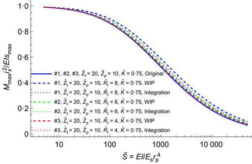
Normalised bending moments for cases #1, #2 and #3, under the different formulations. A full-colour version of this figure can be found on the ICE Virtual Library (www.icevirtuallibrary.com)
Normalised bending moments for cases #1, #2 and #3, under the different formulations. A full-colour version of this figure can be found on the ICE Virtual Library (www.icevirtuallibrary.com)
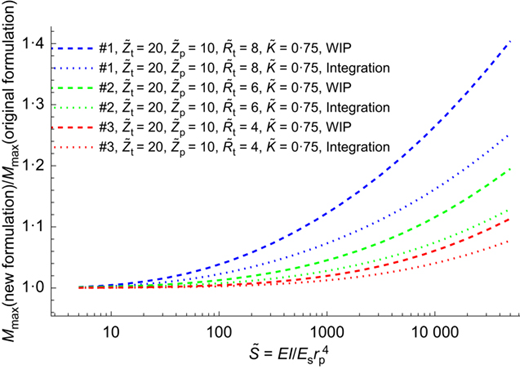
Ratios of bending moment between methods for cases #1, #2 and #3. A full-colour version of this figure can be found on the ICE Virtual Library (www.icevirtuallibrary.com)
Ratios of bending moment between methods for cases #1, #2 and #3. A full-colour version of this figure can be found on the ICE Virtual Library (www.icevirtuallibrary.com)
A simple mechanical explanation can be given for the increased effect of the tunnel constraint with increased pipeline bending stiffness (EI): while the greenfield input tends to bend the pipeline downwards, it is the pipeline stiffness that allows the pipeline to resist the down-drag motion and ‘bounce back’ relatively (trying to restore its original shape). This relative upward motion, however, is resisted by the soil. The addition of the tunnel constraint increases the soil resistance to this restoring motion, hence effectively increasing the soil stiffness locally and reducing relative upward motion, which results in higher bending in the pipe.
This tunnel constraint–soil–pipeline interaction mechanism can also be shown in the bending moment and displacement profiles resulting from the three formulations, as shown in Fig. 4. For the case of the pipeline follows closely the greenfield displacement under the three different assumptions: as the pipeline is flexible, there is no relative pipeline–greenfield motion to propagate relative displacement at the tunnel. For there is already a notable difference between the formulations, where the displacement and bending moment are the largest in the WIP case and smallest in the original formulation. The integration case, representing an advancing constraint with the tunnel construction, provides an intermediate value between the original formulation (ignoring the tunnel) and the WIP case. It is, however, closer to the WIP case.
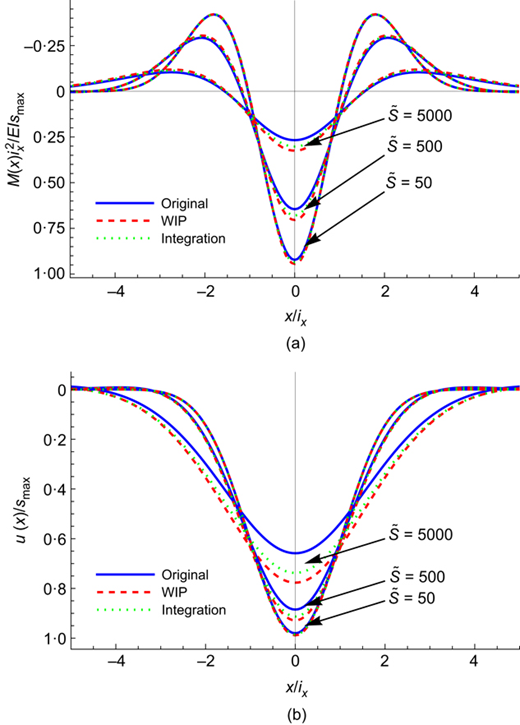
Displacement and bending moment profiles for case #1, for = 50, 500 and 5000: (a) bending moment profiles; (b) displacement profiles
Displacement and bending moment profiles for case #1, for = 50, 500 and 5000: (a) bending moment profiles; (b) displacement profiles
Note, however, that while the difference between the methods becomes greater with stiffness, resulting in a deviation of up to 50% in the bending moments (as illustrated in Fig. 3), their difference from the conservative greenfield analysis approach in which the pipeline is forced to follow the greenfield settlements (which provides Mmax = EIsmax/ix2) is of the same order of magnitude. This suggests that the addition of the tunnel constraint is secondary to the benefits of soil–pipeline interaction when compared to the greenfield approach, yet valuable when performed.
One may consider a simple engineering approximation that relates to this notion of ‘increased soil resistance’. If indeed the tunnel constraint is equivalent to an increase in soil stiffness, then the original approach (with a flexible tunnel) should provide similar values to the constrained continuum approach when the stiffening action of the tunnel is considered with an equivalent (increased) soil stiffness in the original formulation. The use of an increased soil modulus Es in the original approach leads to a horizontal ‘right’ translation (constant shift on the logarithmic plot) of the results presented in Fig. 2.
One may ask what should be the shift (i.e. soil stiffness increase factor) for which the difference between original and constrained continuum predictions is minimised. This can be formulated as
where is the function that provides the normalised maximum bending moment of the new formulation for a given , and is the original formulation, but now used with an increased soil modulus Es = αEs. α* is the optimal α value that brings the integrated squared difference of the relative error to be minimal. In the above minimisation, an equal weight is given for an increment along the log scale of (i.e. ).
For the WIP cases #1, #2 and #3, presented in Fig. 2, it is found that α* is 1·54, 1·21 and 1·11, respectively, with an error of less than 5% over the entire range of considered. This good agreement supports both the engineering explanation for the difference, and that the engineering approximation of ‘increased soil stiffness’ is reasonable. The concept of ‘increased soil stiffness’ is applied in the subsequent section as a simple engineering methodology to establish limits on the impact of the tunnel effect.
Figures 5 and 6 show the comparison between cases #4, #5 and #6 which also vary in but have shallower and but with the same difference as before. While the difference between the methods is slightly larger than that observed in cases #1, #2 and #3, the overall trend is very similar to that observed in the comparison of cases #1, #2 and #3. This is probably due to the fact that the distances between the pipeline and the tunnels are the same (i.e. #4 like #1, #5 like #2 and #6 like #3). The difference is greater because the tunnel constraint is applied on a more flexible (shallow) system and hence enforces greater change.
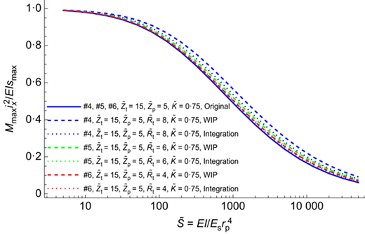
Normalised bending moments for cases #4, #5 and #6, under the different formulations. A full-colour version of this figure can be found on the ICE Virtual Library (www.icevirtuallibrary.com)
Normalised bending moments for cases #4, #5 and #6, under the different formulations. A full-colour version of this figure can be found on the ICE Virtual Library (www.icevirtuallibrary.com)
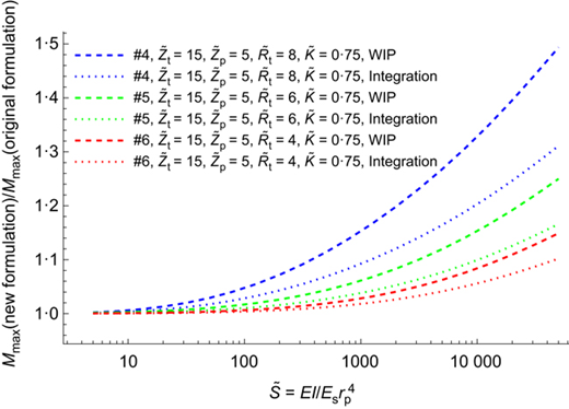
Ratios of bending moment between methods for cases #4, #5 and #6. A full-colour version of this figure can be found on the ICE Virtual Library (www.icevirtuallibrary.com)
Ratios of bending moment between methods for cases #4, #5 and #6. A full-colour version of this figure can be found on the ICE Virtual Library (www.icevirtuallibrary.com)
Figure 7 shows the comparison between cases #5, #7 and #8, which vary in , while Fig. 8 shows the corresponding bending moment ratio between the methods. Unlike the previous sets of comparisons, this one involves a variation of ix/rp, which leads to a significant variation in the resulting bending moment as a function of . Recall that Klar et al. (2005) have used R = EI/Esrpix3 as the relative stiffness parameter for normalisation to eliminate the dependency on ix/rp, but this is unwanted in the current investigation, which aims to identify the governing parameters between the methods. Although the resulting normalised maximum bending moment is highly affected by , the difference between the methods, in terms of moment change, is very similar. This can be clearly seen in Fig. 8 where the lines representing the deviation of the WIP approach from the original method are very similar. In the integration approach, the results are spread. This is most likely because different values also affect the value of iy in equation (14), which was assumed to be equal to ix. That is, smaller also leads to a more abrupt (with tunnel advancement) appearance of the greenfield input, having already a greater tunnel section constructed that adds to the resistance, bringing the results closer to the WIP case.
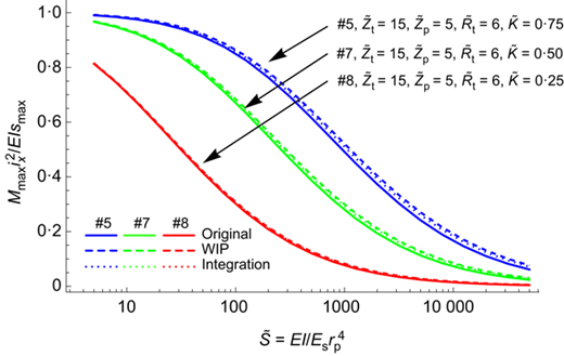
Normalised bending moments for cases #5, #7 and #8, under the different formulations
Normalised bending moments for cases #5, #7 and #8, under the different formulations
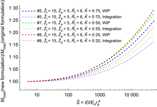
Ratios of bending moment between methods for cases #5, #7 and #8. A full-colour version of this figure can be found on the ICE Virtual Library (www.icevirtuallibrary.com)
Ratios of bending moment between methods for cases #5, #7 and #8. A full-colour version of this figure can be found on the ICE Virtual Library (www.icevirtuallibrary.com)
Considering that does not strongly influence the variation between the methods, it is of interest to ask what may be a suitable parameter, beyond , that quantifies the dependency. From the above investigation, there is clear indication that the separation distance between the pipeline axis and the tunnel crown may be relevant.
This was also evident in the simple engineering approximation of α* where its value decreased with a distance increase between the tunnel crown and the pipeline. It is suggested that the value of α* and the manner in which it changes with could indicate on both the limit of influence and the impact of the tunnel constraint on the results. Such characterisation will also reveal when the more advanced formulation is needed and when the original ‘two-stage’ process is sufficient.
BOUNDS OF THE TUNNEL CONSTRAINTS EFFECT AND A SIMPLE CORRECTION FACTOR
The determination of when the additional constraints become essential and when the original ‘two-stage’ process can suffice is of interest. Building upon insights from the preceding section, the distance between the tunnel crown and the pipeline axis, along with the tunnel radius, could serve as suitable indicators for this determination. In addition, the introduction of α* as a straightforward engineering correction factor to the original method enhances the assessment of tunnel constraint effects.
To examine this hypothesis further, the parametric investigation was extended with the cases presented in Table 2. This parametric study adopts the definition of by Mair et al. (1993) (the equation of which is given in Table 2). Despite this, for design purposes the outcomes in this section in terms of α* are not strictly limited to tunnelling in clays as the influence of on the normalised sagging curvature is limited (see Fig. 8).
Extended cases focusing on radius and distance
| Case | |||||
|---|---|---|---|---|---|
| #9–12 | 20, 18, 16, 14 | 5 | 6 | 5–50 000 | |
| #13–16 | 18, 16, 14, 12 | 5 | 4 | 5–50 000 | |
| #17–20 | 16, 14, 12, 10 | 5 | 2 | 5–50 000 | |
| #21–23 | 20, 18, 16 | 7·5 | 6 | 5–50 000 | |
| #24–26 | 18, 16, 14 | 7·5 | 4 | 5–50 000 | |
| #27–29 | 16, 14, 12 | 7·5 | 2 | 5–50 000 | |
| #30–33 | 16, 14, 12, 10 | 2·5 | 6 | 5–50 000 | |
| #34–37 | 14, 12, 10, 8 | 2·5 | 4 | 5–50 000 | |
| #38–41 | 12, 10, 8, 6 | 2·5 | 2 | 5–50 000 |
For each case considered the α* value was determined by the minimisation problem of equation (16). The current section is focused on the WIP cases, which maximises the role of the constraints on the interaction problem and results in higher α*. As the WIP cases are more conservative than for the other methods, predictions are explored to ask when it may be sufficiently safe to disregard the constraints when evaluating tunnelling-induced stressing – that is, if the WIP does not lead to a significant change in the behaviour so is the tunnel advancement case.
Figure 9 shows the difference between the new formulation (with the constraints) to the original ‘two-stage’ approach as a ratio between the maximum bending moments, while Fig. 10 shows the difference between the approximated engineering approach of increased stiffness () to the new approach. The associated optimal α* values are given in Fig. 11 together with a fitted function. Fig. 10 uses a logarithmic scale for the normalised bending moment to allow evaluation of the relative error of each case. One should recall that although the normalised bending moment decreases with increase in EI (and increase of ), the actual bending moment actually increases. Therefore, the relative error is important also for low values of normalised bending moment. As can be seen, except for cases #37 and #41 in which the tunnel and the pipeline are extremely close (separated by half a pipe radius), the accuracy of the approximation is quite good (less than 5% for the majority of the range considered). One may even say that the approximation is reasonable for #37 and #41, as it reduces the difference between the approaches from a factor of 2 to about 20%.
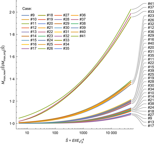
Ratios of bending moment between methods for the cases presented in Table 2. A full-colour version of this figure can be found on the ICE Virtual Library (www.icevirtuallibrary.com)
Ratios of bending moment between methods for the cases presented in Table 2. A full-colour version of this figure can be found on the ICE Virtual Library (www.icevirtuallibrary.com)
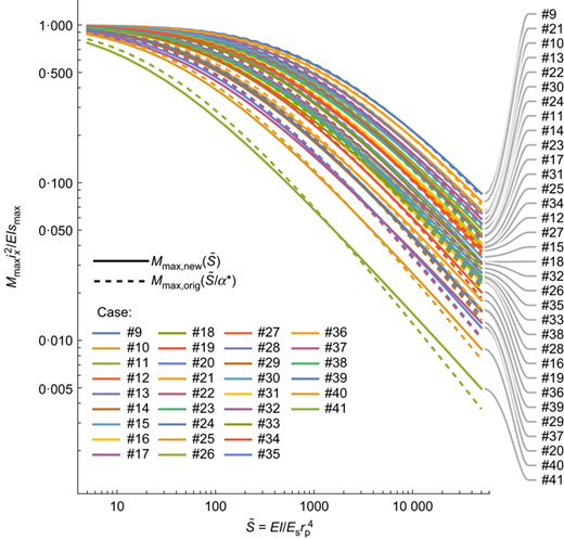
Comparison between ‘shifted’ original formulation using optimal α* and the new kinematic constraint formulation. A full-colour version of this figure can be found on the ICE Virtual Library (www.icevirtuallibrary.com)
Comparison between ‘shifted’ original formulation using optimal α* and the new kinematic constraint formulation. A full-colour version of this figure can be found on the ICE Virtual Library (www.icevirtuallibrary.com)
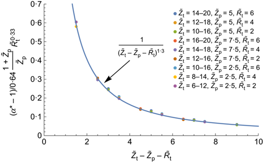
Normalised α* results. A full-colour version of this figure can be found on the ICE Virtual Library (www.icevirtuallibrary.com)
Normalised α* results. A full-colour version of this figure can be found on the ICE Virtual Library (www.icevirtuallibrary.com)
The optimal α* values given in Fig. 11 are plotted in a normalised manner using , and , together with a fitted expression. As can be seen, the agreement with the fitted expression is excellent. As such one can estimate an α* value using:
This expression may be used to quantify the maximum equivalent stiffening of the soil domain in the constrained continuum method, making the original ‘two-stage’ method sufficient for upper and lower estimates of the likely range of induced maximum bending in the pipeline. In addition, it enables the sensitivity of the tunnelling-induced moment to the tunnel's stiffening action to be quantified.
To discuss this objective further, one can adopt the approximated fitted expression for the normalised bending moment of the original formulation as presented in Vorster et al. (2005): Mmaxi2x/smaxEI = 1/(1 + 0·55R2/3). From this relation, the change in the normalised bending moment due to a change in the soil stiffness can be quantified:
where Mn is the normalised bending moment= Mmaxi2x/(smaxEI) derived from the original formulation.
One may consider a criterion for the maximum allowed change in α* to be ignored as a function of the allowed change in the mormalised bending moment defined by a fraction β = dMn/Mn. Considering the above expression this leads to:
This expression, together with equation (17), can be used to decide if the original ‘two-stage’ solution scheme with a fully flexible tunnel is sufficient, or if there is a need for a more advanced continuum analysis considering the tunnel stiffening action:
If the above inequality holds, then the expected change in the stressing would be smaller than β, and thus there is no need to consider the tunnel constraints. However, if the inequality does not hold, one can perform the more advanced constraint analysis or use the estimated α* with the original formulation for evaluation of the maximum bending moment.
The trends of the above inequality are worth discussing. In the case when Mn is close to 1, the right-hand side approaches zero and the inequality will hold. This is because the pipeline simply follows the soil and a greater soil stiffness would not change that condition by much. The smaller β is, the greater the right-hand side, and the greater the chances for violating the inequality (i.e. that the difference between the methods will exceed the accepted error threshold). Regardless of the distance between the tunnel and the pipeline, larger tunnels lead to a smaller left-hand side, (i.e. a greater chance to violate the inequality).
The above inequality is clearly approximated, both because it is based on the derivative assumption which is valid for small changes in Es and also because it involves an approximated relation between R and Mn (i.e. the Vorster et al. (2005) expression) as well as the approximated engineering approach of utilising α* as a correction factor to the soil stiffness. Nonetheless, it still provides a valuable engineering tool for quick assessment when the ‘two-stage’ method is sufficient. The appendix shows an example of its use.
SUMMARY AND CONCLUSION
This paper has extended the classical elastic continuum matrix-based analysis of soil–pipeline interaction due to tunnelling-induced soil deformations by introducing, into the formulation, constraints resulting from the presence of a rigid tunnel. In other words, the classical analysis method assumed the tunnel as fully flexible. While still relying on an input of the form of greenfield displacement, the formulation presented in this paper considers all of the components involved in the problem; therefore, it may be referred to as a solution for tunnel–soil–pipeline interaction in which the tunnel stiffening action of the continuum domain is accounted for. As such, the formulation also requires details about the tunnel location and diameter, and not merely the greenfield input. The final matrix-based set of equations has a very similar structure to the original formulation, only that the λ*s is updated using a new closed-form set of expressions.
A parametric investigation was performed to evaluate the impact of including the tunnel constraints (as vertical fixities at the tunnel periphery) in the formulation. It was found that the existence of tunnel constraints leads to higher bending stressing in the pipeline, and is more conservative than the original approach. In particular, two boundary conditions were studied for the rigid tunnel: WIP constraints for the entire tunnel (with steady-state greenfield movements) and an advancing tunnel with constraints behind the tunnel face (considering the transient evolution of greenfield movements). The fully flexible and WIP tunnel solutions are expected to bracket the realistic intermediate case. A simple engineering approximation was suggested for the effect of the additional constraints, being equivalent to having a stiffer soil (i.e. increased soil modulus by a factor of α*).
The question when and if the tunnel constraints can be ignored was also addressed, with a result of a simple-to-use inequality involving the tunnel diameter and the relative pipe-to-tunnel distance, against the normalised bending moment and an accepted level of deviation from the classical analysis for a fully flexible tunnel.
Although the addition of the tunnel constraint to the solution can lead to a substantial increase in the bending moments, the difference between the original method and the new one compared to the conservative greenfield analysis approach of ‘forcing the pipeline to follow the greenfield settlements’ is of the same order of magnitude. While this infers that the tunnel constraint is secondary to the overall benefits of soil–pipeline interaction when compared to the greenfield engineering approach, it is still significant within the soil–pipeline interaction analysis for cases with high relative pipeline soil stiffness.
While the presented technique was applied to the problem of tunnelling effects on pipelines, its applicability extends to other ‘two-stage’ methods. For instance, it could be seamlessly adapted for analysing tunnelling effects on buildings, showcasing the versatility and broad utility of the proposed approach.
Data availability statement
The data supporting this study can be found within the paper, and guidance on the implementation of the equations is available upon request from the corresponding author and in the online supplementary material.
ACKNOWLEDGEMENTS
This research was supported by the Israel Science Foundation (grant no. 1425/23). The idea for the paper emerged from discussions held while the first author visited Tongji University under the Chinese governmental Foreign Expert Exchange Program (G2022133013l).
NOTATION
- cp
cover depth of the pipe
- ct
cover depth of the tunnel
- dp
diameter of the pipe
- dt
diameter of the tunnel
- EI
flexural rigidity of the pipe
- Es
Young's modulus of the soil
- F
force vector representing soil loading on the pipe
- Ft
tunnel reaction forces
- f
forces acting on the soil medium along the pipe
- Gi,j
Green's function
- ix
settlement trough width parameter
- iy
settlement trough length parameter
- K*
local soil stiffness matrix
width parameter
- Mmax
maximum bending moment
- Mn
normalised maximum bending moment
- R
original relative pipe soil stiffness
ratio of tunnel to pipe radii
- rp
radius of the pipe
- rt
radius of the tunnel
alternative pipe soil relative stiffness
- S
stiffness matrix of the pipe
- smax
maximum greenfield settlement
- sv(x, y)
three-dimensional settlement trough
- u
pipeline displacement
- uC
soil continuum displacement
- uCA
additional displacement at a point due to forces acting at other places
- uCAP
additional displacement resulting from forces of soil–pipe interaction
- uCAT
additional displacement resulting from tunnel
- ugf
greenfield displacement
- uR
displacement along the pipeline due to reaction of the tunnel
- ut
displacement at points along the tunnel due to pipeline interaction forces
- x
transverse distance from the tunnel
- y
distance ahead of the tunnel face
normalised pipe depth
normalised tunnel depth
- zp
depth of the pipe
- zt
depth of the tunnel
- α*
optimal equivalent increase in soil stiffness
- β
restricted error
- ΔL
‘back-shift’ of effective tunnel face location
- λ′
pipe tunnel flexibility matrix
- λ*s
original soil interaction matrix
- λ**s
update soil continuum interaction matrix
- λtt
tunnel flexibility matrix
REFERENCES
APPENDIX. EXAMPLE USE OF THE INEQUALITY AND THE APPROXIMATION
Consider a 2 m dia. pipeline with an EI = 8 × 10⁶ kNm2 buried at a depth of 5 m (i.e. ). A 6 m dia. tunnel is being excavated at a depth of 10 m (i.e. and ). The soil stiffness is estimated to be Es = 50 MPa. Consequently, the value of . based on Mair et al. (1993). Performing the analysis with the original formulation provides a normalised bending moment of Mn = 0·37. For the sake of the example, it is suggested that an error of β = 5% is acceptable, in which case the inequality of equation (20) turns out to be 1·42 > 5·37, which does not hold, and infers that the tunnel constraints need to be considered. Using equation (17) to estimate α* results in α* = 1·44. Introducing this value to the original ‘two-stage’ formulation with , results in Mn = 0·43. This value is indeed close to the output of the new formulation (with the tunnel constraints) under , which provides Mn = 0·41 (difference less than 5%).
The example can be repeated for a case where the soil stiffness is estimated to be much lower, say Es = 10 MPa. In this case the and the original formulation provides a normalised bending moment of Mn = 0·16. Returning with this value to the inequality, equation (20), again with β = 5% results in 1·42 > 7·16, which does not hold. The α* is the same as before, = 1·44, as it is governed only by the geometry. Using it to approximate the response with the constraints by using together with the original formulation provides Mn = 0·20, which is quite similar to the new formulation output under (which provides Mn = 0·19). Note that the difference between the two formulations is greater in the second case of the softer soil (0·19/0·16 as opposed to 0·41/0·37), because the relative effect of the constraints is more substantial in this case.
The above two examples constitute cases in which the inequality does not hold when β = 5%. If, for example, the tunnel was positioned at a greater depth, say 15 m instead of 10 m, then Mn = 0·68 and Mn = 0·39 for and , respectively, based on the original ‘two-stage’ method (note that in this case ). In this case, of a deeper tunnel, the inequalities are 7·27 > 2·81 for the stiff soil case () and 7·27 > 5·20 for the soft soil case (. In both cases the inequality holds, suggesting there is no need for more advanced analysis. In fact, performing the analysis with the new kinematic constraint approach yields Mn = 0·68 for the first case and Mn = 0·40 for the second case, both of which are very close to the original ‘two-stage’ method solution.
Discussion on this paper closes 1 May 2026; for further details see p. ii.

