


A laboratory study was carried out on a sandy silt gold tailings to investigate the effect of the Lode angle (θ) on the critical state line (CSL) in the compression (e–p′) and effective stress (q–p′) planes, and to study the strength anisotropy of the tailings. Four sets of strain-controlled tests were carried out: (a) drained and undrained triaxial compression tests; (b) torsional shear hollow cylinder tests under drained and undrained conditions at constant θ and constant direction of the major principal stress relative to the vertical axis (α); (c) drained and undrained triaxial extension tests; and (d) undrained hollow cylinder simple shear tests. The tests were carried out on loose moist tamped (LMT) and dense slurry air-dried (AD) prepared specimens. The results indicated that: (a) the CSL in the compression plane does not depend on θ or on the stress path; (b) the stress-dilatancy is dependent on θ while the effect of θ on state-dilatancy is minor; (c) the undrained yield strength of LMT was found not to depend significantly on the state parameter (ψ), but it was significantly affected by the stress path followed during consolidation and subsequent shear, for example, by the pre-shearing stress ratio, stress-reversal loading, θ and α. The results demonstrate the contribution of the initial shear stress and evolving anisotropy on the undrained strength of the gold tailings in a loose state.
NOTATION
- B
Skempton’s pore pressure coefficient
- bias
static horizontal shear stress ratio = τzϑ/
- e
void ratio
- e0, λc, ξ, pref
critical state line e–p′ constants
- G
shear modulus
- H
initial sample height
- K
bulk modulus
- Kc
principal stress ratio =
- k
slope of isotropic unloading consolidation line
- M
critical friction ratio general stress conditions
- MT
torque
- N
volumetric coupling parameter
- Pi, Po
inner and outer pressures
- ro, ri
outer and inner radii
- uo, ui
outer and inner radial displacements
- W
axial load
- β
angle between the vertical axis and the direction of trimming of the air-dried specimens
- η
stress ratio = q/p′
- Θ
angle of rotation in torsional shear hollow cylinder
- θ
Lode’s angle
- ν
Poisson’s ratio
- χ
state-dilatancy coefficient
- ψ
state parameter
Subscripts
INTRODUCTION
The last decade has seen the static liquefaction failure of several tailings storage facilities (TSFs) containing loose/saturated fills, for example the Fundão (Morgenstern et al., 2016), Cadia (Jefferies et al., 2019) and Feijão (Robertson et al., 2019; Arroyo & Gens, 2021) TSFs. These failures caused substantial economic and environmental damage and highlighted the importance of using a robust approach for assessing the failure risk of these structures based on critical state soil mechanics (CSSM) (Jefferies, 2022). Analysis of TSFs through CSSM has recently gained significant attention as this provides a more robust evaluation of the risk of liquefaction of tailings than methods based solely on empiricism. In this context, the evaluation of the critical state line (CSL) and the determination of the in situ state parameter (ψ – Been & Jefferies, 1985) have become key inputs to these analyses.
The standard method to define the CSL in the compression plane (e–p′) and effective stress plane (q–p′) is under triaxial compression (TC) loading conditions. An assumption typically adopted in CSSM is that the CSL in the e–p′ plane is unique – that is, independent of density, anisotropy and stress path. This assumption has been deduced from experimental work (e.g. Been et al., 1991; Schnaid et al., 2013; Salvatore et al., 2017; Becker et al., 2022), by way of thermodynamic principles and numerically (Li & Dafalias, 2012). However, there is some experimental work (e.g. Wanatowski & Chu, 2007; Wagner et al., 2023) and numerical evidence (e.g. Huang et al., 2014; Zhu et al., 2024) to suggest that the CSL in the e–p′ plane may depend on the magnitude of the intermediate principal stress (σ2) with respect to the other principal stresses (major σ1, minor σ3), a stress parameter often defined by the Lode angle (θ) (Lode, 1926) or the intermediate principal stress ratio (b) (Habib, 1953), and by the pre-shearing stress ratio (Kc) (Fotovvat & Sadrekarimi, 2022). Hence, this topic remains unresolved.
The CSL in the compression plane being dependent on θ could have important implications for the estimation of key tailings strength parameters – such as the stress ratio at instability (ηIL) (Lade, 1992), the peak undrained shear strength ratio and the post-liquefaction undrained shear strength ratio – as these parameters are typically correlated to ψ (e.g. Jefferies & Been, 2016). This is particularly important as most stability problems of slopes are plane strain, where θ and the direction of the major principal stress (σ1) relative to the vertical axis (α) deviate from TC conditions. The potential effect of a CSL e–p′ that is dependent on θ on the post-liquefaction strength is schematically illustrated in Fig. 1 for a material in a loose state. In this example, the CSL e–p′ measured in TC is located between two hypothetical CSL e–p′ relations measured at a particular θ, and for simplicity it is assumed that all CSL e–p′ relations are parallel and follow a semi-log idealisation (Fig. 1(a)). Under this very loose state, the post-liquefaction strength is assumed to be equal to the strength at critical state and, as such, if the CSL e–p′ is dependent on θ, its post-liquefaction strength will also depend on θ. This concept can be clearly deduced from Fig. 1(b), wherein the behaviour of the loose material shearing towards its critical state is illustrated in the q–p′ plane for the three CSL e–p′ scenarios. In order to focus attention only on the effect that a CSL e–p′ dependent on θ could have on the strength at critical state, the deviatoric stress q is normalised by p′ at consolidation () and by the ratio M/MTC, wherein M (critical state friction ratio) is the slope of the CSL in the q–p′ plane at a generic θ and MTC is the slope of the CSL in TC loading. By adopting this normalisation, the influence of M with θ is removed and the strength at critical state can be calculated using the equation derived by Jefferies & Been (2016), adopting the state parameter measured on the CSL e–p′ at the relevant θ(ψ0_θ). From Fig. 1, it is clear that if the CSL e–p′ dependent on θ is higher than the TC CSL, the strength at critical state would be greater than that measured in TC, for example, as was found by Wanatowski & Chu (2007). However, the exact opposite would occur if the CSL e–p′ dependent on θ is lower than the TC CSL e–p′, for example, as reported by Wagner et al. (2023). Such differences could have enormous safety or cost implications when assessing the stability of TSFs under post-liquefaction strength conditions.
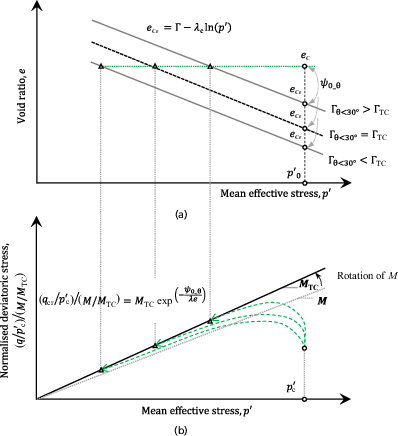
Schematic representation of the effect of a CSL e–p′ dependent on θ on the post-liquefaction strength (critical state) of loose contractive materials: (a) e–p′ plane and (b) normalised q–p′ plane
Schematic representation of the effect of a CSL e–p′ dependent on θ on the post-liquefaction strength (critical state) of loose contractive materials: (a) e–p′ plane and (b) normalised q–p′ plane
Several experimental works on geomaterials prepared in loose and dense states have clearly indicated the dependency of the peak friction ratio (ηp) and M on θ (e.g. Matsuoka & Nakai, 1974; Van Eekelen, 1980; Ochiai & Lade, 1983; Wanatowski, 2005; Jefferies & Shuttle, 2011). However, laboratory data defining comprehensively the dilatancy of geomaterials under various values of θ, densities, stress levels and drainage conditions, and at the same time rationalised in terms of a CSSM framework, are limited. The exceptions are the data synthesised by Jefferies & Shuttle (2002, 2011) based on Cornforth (1961, 1964) and Wanatowski & Chu (2007), the experimental testing carried out by Been et al. (1991), Wanatowski (2005), Wanatowski & Chu (2007), Schnaid et al. (2013), Salvatore et al. (2017), Fotovvat & Sadrekarimi (2022), Becker et al. (2022) and Wagner et al. (2023). Of these experimental data only the work of Cornforth and Wanatowski included testing relevant to plane strain loading, while the other cited research focused on comparing TC to triaxial extension (TE) loading. Further, only the work of Schnaid et al. (2013), Fotovvat & Sadrekarimi (2022), Becker et al. (2022) and Wagner et al. (2023) studied tailings, while the others investigated natural sands. This highlights the need for more studies focusing on tailings, including testing at conditions relevant to below-slope conditions.
Soil anisotropy is typically defined by three components (Ladd, 1991): inherent or fabric, initial shear stress and induced or evolving anisotropy. Inherent anisotropy relates to the microlevel (e.g. particle orientation) and macrolevel (e.g. layering) structure of a material. Initial shear stress anisotropy is typical of level ground conditions, wherein consolidation occurs under K0 compression loading conditions. Induced anisotropy may manifest in sloping ground conditions, and it is relevant to structures like TSFs, which are constructed in stages. Under induced anisotropy, the initial anisotropy of a material (inherent and initial shear stress) changes due to plastic strains resulting from stresses (consolidation and shear) applied progressively during staged construction (Ladd, 1991), causing a potential rearrangement of particle contact (e.g. Wong & Arthur, 1985). The effects of anisotropy on the drained and undrained stress–strain behaviour of geomaterials has been investigated in various experimental works in the directional shear cell (DSC) (e.g. Arthur & Menzies, 1972; Wong & Arthur, 1985), true triaxial (TT) (e.g. Yamada & Ishihara, 1979; Ochiai & Lade, 1983), torsional shear hollow cylinder (TSHC) (e.g. Shibuya, 1985; Uthayakumar, 1996; Yoshimine et al., 1998; Sivathayalan & Vaid, 2002; Bahadori et al., 2008; Fanni et al., 2022, 2024; Reid et al., 2022a), through comparison of data obtained from various testing devices (e.g. Ladd, 1991; Sadrekarimi, 2016; Fotovvat & Sadrekarimi, 2022) and numerically (Li & Dafalias, 2012; Salimi & Lashkari, 2020; Wang et al., 2020). Drained DSC and TT testing indicated that anisotropy could affect the stress–strain behaviour of dense sands (e.g. Ochiai & Lade, 1983,; Wong & Arthur, 1985). These findings were later confirmed in discrete-element method (DEM) simulations by Salimi & Lashkari (2020) and Wang et al. (2020). Regarding the liquefaction risk, the TSHC testing and DEM simulations of Salimi and Lashkari indicated that the instability of anisotropic materials depends on the shearing loading conditions (θ and α) in respect of the bedding plane (angle of particle alignment) with flow liquefaction susceptibility increasing as θ and α deviate from TC conditions.
Owing to the paucity of testing on tailings and the uncertainties previously outlined, there is a need to investigate the mechanical behaviour of tailings to (a) assess if the CSL e–p′ may depend on θ; (b) determine stress- and state-dilatancy parameters at various values of θ: and (c) better understand the effect of anisotropy on instability. In order to address these aspects, laboratory testing was carried out on a sandy silt gold tailings characterised in previous studies (e.g. Ayala et al., 2020; Reid et al., 2021, 2022b; Fanni et al., 2022, 2023). The testing consisted of drained/undrained TC (i.e. TC: θ = 30° or b = 0, α = 0°) and extension testing (i.e. TE: θ = −30° or b = 1, α = 90°) with and without stress reversal, drained/undrained TSHC at θ = 0° (b = 0·5), α = 45° and undrained hollow cylinder simple shear (HCSS) tests. The HCSS tests were carried out with and without the application of a static horizontal shear stress (commonly referred to as ‘bias’) to investigate the effect of below-slope stress conditions on the undrained behaviour of the tailings. To complement the experimental study, resonant column (RC) tests were carried out to measure the small-strain stiffness of the tailings.
All specimens were prepared in a loose state using the loose moist tamping (LMT) technique and in a dense state from specimens trimmed from blocks manufactured by pouring a non-segregating thickened slurry into a container, followed by being air-dried (AD) (Reid et al., 2022c,; 2024; Fanni et al., 2023). The LMT procedure was used to allow inference of the CSL e–p′, owing to the propensity of a specimen in a loose initial state to be less prone to localisation than dense specimens (e.g. Desrues et al., 1996; Jefferies & Been, 2016; Salvatore et al., 2017). Both LMT and AD procedures were adopted to infer stress- and state-dilatancy parameters, while the effect of anisotropy on the undrained strength of the gold tailings was based on the LMT tests, with shearing carried out following various stress-paths. Trimming of the AD specimens was undertaken at 0° and 90° directions with respect to the vertical axis (β) (which also represents the direction of slurry deposition). This was done to investigate the inherent anisotropy of AD specimens’ effects on stress- and state-dilatancy. Only drained TE tests were carried out using AD with β = 0° and 90°, while the other tests used AD specimens with β = 0°. The data produced in this study were complemented by the HCSS of Fanni et al. (2022) and TSHC TC testing of Fanni et al. (2023) and Reid et al. (2021, 2022b, 2023, 2024).
MATERIALS AND METHODS
Materials
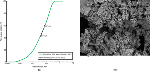
The material used in this study is a low-plasticity sand–silt gold tailings (Ayala et al., 2020; Fanni et al., 2022,, 2023; Reid et al., 2022b). The tailings have a specific gravity of 2·78, 59% particles <75 μm and 43% particles <38 μm, liquid limit (LL) of 18% and plasticity index (PI) of 2%. The particle size distribution (PSD) by laser sizing carried out by Reid et al. (2021) is reported in Fig. 2 along with the particles retained on the 75 and 38 μm sieves for the material used in this study. Semi-quantitative X-ray diffraction (XRD) testing carried out by Ayala et al. (2020) indicated that the main minerals are quartz (33%), albite (26%), muscovite (12%), clinochlore (11%) and biotite (10%). The particle morphology, shown in Fig. 2, indicates the presence of particles of very angular shape, low sphericity and low roundness within the entire particle size range (sand and silt sizes), with aspect ratio varying across the particle size spectrum from approximately 1 to 8. Typically, the particles with the greatest aspect ratio are of sand and coarse silt size, while fine silt particles are more likely to have an aspect ratio tending towards 1. This difference in aspect ratio between sand and silt size particles can be attributed to the way ore is processed by crushing at the mine processing plant.
Specimen preparation
Specimens were prepared adopting the LMT and AD preparation methods. These two approaches were selected to provide a range of states while avoiding the potential for tamping-induced overconsolidation of specimens when targeting dense states (Reid et al., 2022b, 2022d).
The TSHC LMT specimens were prepared by moist tamping in ten layers of equal volume at a gravimetric water content (GWC) of 10%, applying an undercompaction ratio (Ladd, 1978) of 5%, to a height of 200 mm with outer and inner diameters of 100 mm and 60 mm, respectively. The LMT specimens were tamped using a specially designed tamping apparatus, wherein the tamper has a donut shape and allows, by adjusting the rod height, the target layer height to be achieved (Fanni et al., 2022, 2023, 2024). After tamping, an isotropic stress by way of suction of approximately 50 kPa was applied to allow removal of the split mould and setting up of the specimen for saturation. The LMT specimens for the resonant column and triaxial tests were prepared in a similar manner but tamped in eight layers to typically a height and diameter of 145 mm and 72 mm, respectively. The AD technique comprised pouring a non-segregating thick slurry at a GWC of 40% into a bucket and vibration to various degrees, followed by a period of drying at a temperature of <50°C, and finally trimming (Fanni et al., 2023).
TSHC testing procedure
TSHC tests were carried out in a device manufactured by GDS Instruments (UK). The cell, inner and back pressures/volumes were measured or controlled by pressure volume controllers (PVCs), while a submersible multiaxial load cell located at the top of the specimen measured the torque and axial load. Two load cells were adopted in this study depending on the target stress, that is 30 Nm/3 kN (low stress) and 200 Nm/20 kN (high stress). Details of the TSHC device and instrumentation used in the tests are provided in Fanni et al. (2022a, 2022b, 2023), as well as in Reid et al. (2022a).
The θ and α values of 0° and 45° adopted in some of the TSHC tests were selected because this stress condition produces a uniform stress distribution across the hollow cylinder wall (e.g. Hight et al., 1983; Saada, 1988; Vaid et al., 1990) – hence reducing stress and strain non-uniformities – and also because it provides θ in between TC and TE loading.
The undrained HCSS tests were carried out adopting the method used by Ampadu (1991), Pradhan et al. (1988), Menkiti (1995) and Fanni et al. (2022) by consolidating with and without the application of a bias (τzϑ/).
All specimens were flushed with deionised water and back-pressure saturated maintaining an effective stress of typically 50 kPa, to achieve a Skempton’s coefficient B ≥98%. Consolidation was then carried out either isotropically or anisotropically to the target stress. Drained and undrained shearing was carried out at a strain rate (axial strain rate, , or horizontal shear strain rate, , depending on the test type) equal to a maximum 2%/h.
The void ratio was calculated using a variation of the end of test (EoT) freezing method proposed by Sladen & Handford (1987), as outlined in Fanni et al. (2023), which indicated accuracy in e < 0·02. This accuracy is within those reported by others when the EoT method with freezing has been adopted for triaxial testing (Reid et al., 2021).
Resonant column testing procedure
The RC tests were carried out on LMT and AD specimens in a Stokoe-type apparatus manufactured by GDS Instruments. The specimens were saturated following the same procedure outlined for the TSHC test. Consolidation was then carried out isotropically in stages. At the end of each consolidation stage and following a period of creep of approximately 4 h, a resonant excitation was provided to the specimens by way of magnetic coils and the small-strain shear modulus (Gmax) was measured at each stage of consolidation. Unloading and reloading (U/R) stages were carried out at various stresses to enable calculation of the small-strain bulk modulus (Kmax).
Three RC tests were carried out, two on LMT and one on AD specimens. RC stages on the first LMT could be carried out only up to p′ = 100 kPa, as the specimen tilted during saturation and consolidation, preventing continuation of RC testing. Isotropic U/R loops were performed on this specimen in stages up to p′ = 400 kPa. In a similar way to the first LMT specimen, the second LMT specimen also tilted when consolidated to p′ = 100 kPa. To allow further RC stages to be carried out on this specimen, the cell and back-pressures were reduced, the device was opened and the specimen levelled off so that RC testing could be continued to p′ = 600 kPa. The void ratio of the RC specimens was calculated using the EoT freezing method (Sladen & Handford, 1987).
Triaxial compression and extension testing procedure
The TC and TE testing was carried out on LMT and AD specimens by using oversized lubricated platens and EoT soil freezing to provide accurate measurement of void ratio. Lubrication of the TC platens was provided by applying two layers of high-vacuum silicon grease between latex membranes and platens (e.g. Tatsuoka et al., 1984; Lam & Tatsuoka, 1988; Jefferies & Been, 2016) while the TE tests were carried out using one lubricated layer (Lam & Tatsuoka, 1988). The specimens were saturated following the same procedure outlined for the TSHC tests, anisotropically consolidated and sheared under drained or undrained conditions at equal to maximum 2%/h.
Definition of stresses and strains
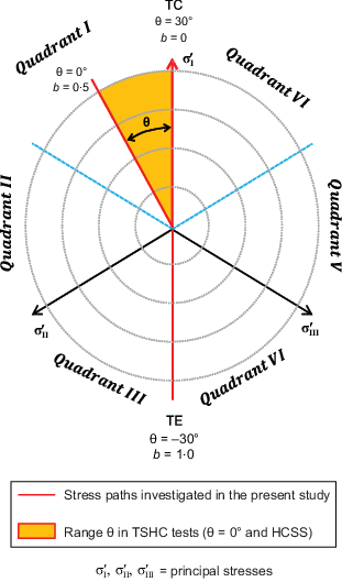
The general stress conditions in the TSHC specimen are presented in Fig. 3, while the equations used to define the stresses and strains in the TSHC and triaxial testing are provided in Table 1. The angle α is defined with respect to the vertical axis, which for the tailings studied represents the depositional axis of the particles (refer to Fig. 3). The stress paths investigated with respect to θ are shown schematically in Fig. 4 in the π-plane representation. The angle θ is calculated adopting the formulation by Ochiai & Lade (1983), although corrected so that TC corresponds to +30° (b = 0) and TE to −30° (b = 1) (e.g. Jefferies & Shuttle, 2002, 2011), with this range maintained in each quadrant of the π-plane representation. The behaviour of cross-anisotropic materials is typically symmetric with respect of the right and left quadrants (e.g. Ochiai & Lade, 1983), hence, typically only one side of the π-plane is investigated.
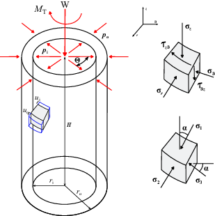
Stress conditions in torsional shear hollow cylinder (adapted from Hight et al. (1983) and Fanni et al. (2022, 2024))
Stress conditions in torsional shear hollow cylinder (adapted from Hight et al. (1983) and Fanni et al. (2022, 2024))
Stress and strain equations (TSHC and triaxial)
| Parameter definition | Stresses | Strains |
|---|---|---|
| Vertical | ||
| Radial | ||
| Circumferential | ||
| Shear | ||
| Major principal | ||
| Intermediate principal | σ2 = σr | ε2 = εr |
| Minor principal | ||
| Deviatoric stress/strain | ||
| Mean effective stress | — | |
| Intermediate principal stress ratio | — | |
| Lode angle | — | |
| Direction of the major principal stress relative to the vertical axis | α = 45° if σz = σϑ | — |
| Stress ratio | — | |
| Volumetric strain | — | |
| Dilatancy |
RESULTS
Elasticity parameters
The RC tests are presented in Fig. 5(a) by plotting the Gmax against p′ normalised by a reference stress (pref) equal to 100 kPa. The data were fitted to an idealisation (equation (1)) similar to that adopted by Shuttle & Jefferies (2016).
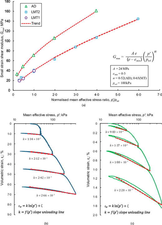
RC: (a) AD and LMT Gmax plotted against /pref data and fitting trends; also unload and reload isotropic consolidation loops for (b) LMT and (c) AD
RC: (a) AD and LMT Gmax plotted against /pref data and fitting trends; also unload and reload isotropic consolidation loops for (b) LMT and (c) AD
The fitting parameters A and emin were found to be the same for both LMT and AD (A = 24 MPa and emin = 0·3). However, the exponent n differed slightly, with n = 0·65 for LMT and n = 0·52 for AD, which may be attributed to differences in fabric between LMT and AD. The greater Gmax observed for AD within the entire stress range is attributed to the greater density of AD compared to LMT. This stiffness difference can also be observed from the response of LMT and AD to isotropic consolidation (Figs 5(b) and 5(c)), wherein the εv of LMT is ≈ 3–4 greater than the εv of AD.
To infer a second elastic parameter required to define the elastic behaviour of the tailings, the isotropic unloading stage was used to calculate Kmax by fitting a semi-logarithmic idealisation (equation (2)) to the data.
The Kmax values reported are for stresses at the onset of unloading and were calculated adopting a mean effective stress difference kPa and the slope of the isotropic unloading consolidation line (k). Poisson’s ratio (ν) was calculated using the typical elasticity equation (equation (3)), and it was found that ν ranged between 0·12 and 0·16 for AD and between 0·17 and 0·21 for LMT.
The elasticity parameters deduced from the tests are summarised in Table 2.
Summary data from resonant column testing
| Test ID | p′: kPa | e | k | Kmax: MPa | Gmax: MPa | v |
|---|---|---|---|---|---|---|
| LMT1 | 30 | 0·791 | — | — | 20 | — |
| 48 | 0·774 | 1·34 × 10−3 | 34 | 24 | 0·21 | |
| 98 | 0·737 | 2·12 × 10−3 | 46 | 40 | 0·17 | |
| 198 | 0·700 | 2·42 × 10−3 | 82 | 66 | 0·18 | |
| 398 | 0·667 | 2·66 × 10−3 | 149 | 107 | 0·21 | |
| LMT2 | 28 | 0·773 | — | — | 21 | — |
| 99 | 0·743 | — | — | 38 | — | |
| 38 | 0·702 | — | — | 26 | — | |
| 100 | 0·697 | — | — | 41 | — | |
| 198 | 0·685 | — | — | 63 | — | |
| 298 | 0·670 | — | — | 88 | — | |
| 398 | 0·659 | — | — | 107 | — | |
| 596 | 0·641 | — | — | 145 | — | |
| AD1 | 18 | 0·459 | — | — | 33 | — |
| 46 | 0·457 | 9·83 × 10−4 | 49 | 49 | 0·13 | |
| 98 | 0·451 | 1·37 × 10−3 | 72 | 71 | 0·13 | |
| 196 | 0·444 | 1·88 × 10−3 | 105 | 106 | 0·12 | |
| 396 | 0·433 | 2·20 × 10−3 | 181 | 161 | 0·16 |
It is acknowledged that the use of two stiffness parameters represents a simplification, as most soils require five stiffness components to define their elastic response in any direction (e.g. Wood, 1990). In this study, the stiffness measured in the RC represents the shear modulus in the horizontal plane (Gmax,vh), while the Kmax may be considered an average stiffness that reflects the contribution of both horizontal and vertical stiffness components.
Stress–strain behaviour
The stress–strain behaviour of the drained tests carried out on LMT and AD at TC, θ = 0°, α = 45° and TE loading is provided in Fig. 6 while the behaviour of the undrained tests at TC, TE, θ = 0°, α = 45° and HCSS loading on LMT specimens is provided in Fig. 7. States recorded during various stages of the tests are summarised in Table 3 (TC), Table 4 (θ = 0° α = 45°), Table 5 (TE) and Table 6 (HCSS). To allow easy identification of the TE results and to adopt typical plotting of TE in the literature, a negative sign was assigned to the deviatoric stress in TE. The results show that LMT contracted under drained conditions, indicating volumetric strains (εv) ranging between +2% and +7%, while AD exhibited a small or negligible contraction followed by dilation. The undrained tests on LMT were carried out on specimens with ψ0 ranging between +0·09 and +0·04. All tests except one (i.e. TSHC-TC LMT-05 at ψ0 = +0·04) exhibited positive excess pore pressure (Δu) and strain-softening behaviour typical of materials susceptible to liquefaction, wherein the tests show post-peak strength loss characterised by a monotonic decrease of q to a minimum strength (i.e. the post-liquefaction strength). TSHC-TC LMT-05 exhibited a post-peak strength loss followed by limited strain-hardening behaviour, where the local minimum q is referred as the quasi-steady state (QSS) (e.g. Alarcon-Guzman et al., 1988).
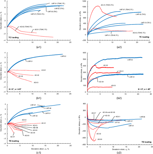
Stress–strain behaviour drained tests: (a1), (a2) TC; (b1), (b2) θ = 0° (b = 0·5) α = 45°; and (c1), (c2) TE
Stress–strain behaviour drained tests: (a1), (a2) TC; (b1), (b2) θ = 0° (b = 0·5) α = 45°; and (c1), (c2) TE
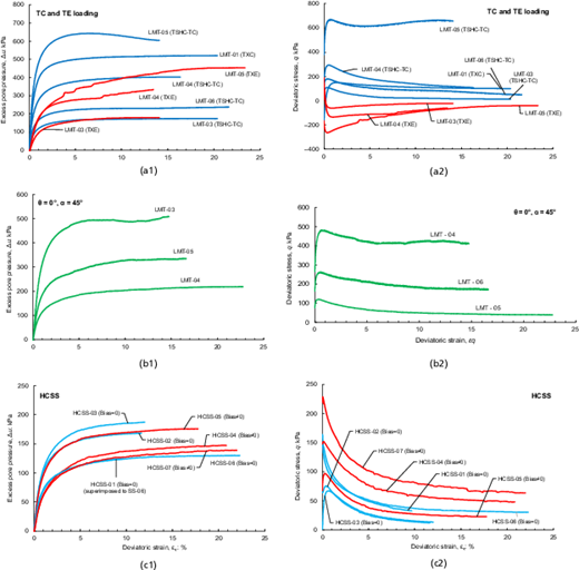
Stress–strain behaviour undrained tests: (a1), (a2) TC and TE; (b1), (b2) θ = 0° (b = 0·5) α = 45°; and (c1), (c2) HCSS
Stress–strain behaviour undrained tests: (a1), (a2) TC and TE; (b1), (b2) θ = 0° (b = 0·5) α = 45°; and (c1), (c2) HCSS
Triaxial compression loading (AD block β = 0°)
| Test ID | Device | Test type | Consolidated states | End of test states | Critical states | ||||||||
|---|---|---|---|---|---|---|---|---|---|---|---|---|---|
| α: deg | θ: deg | ec | : kPa | qc: kPa | e | p′: kPa | q: kPa | ecr | : kPa | Qcr: kPa | |||
| Fanni et al. (2023) | |||||||||||||
| LMT-01 | TSHC | CID | 0 | 30 | 0·764 | 51 | 1 | 0·638 | 90 | 122 | 0·638 | 90 | 122 |
| LMT-02 | CID | 0·714 | 150 | 1 | 0·600 | 280 | 390 | 0·600 | 280 | 390 | |||
| LMT-03 | CAU | 0·698 | 200 | 60 | 0·698 | 8 | 9 | 0·698 | 8 | 9 | |||
| LMT-04 | CAU | 0·637 | 500 | 150 | 0·637 | 84 | 107 | 0·637 | 84 | 107 | |||
| LMT-05 | CAU | 0·562 | 1002 | 380 | 0·562 | 490 | 656 | 0·562 | 490 | 656 | |||
| LMT-06 | CAU | 0·655 | 299 | 111 | 0·655 | 41 | 50 | 0·655 | 41 | 50 | |||
| LMT-07 | CID | 0·650 | 302 | 6 | 0·566 | 551 | 753 | 0·566 | 551 | 753 | |||
| AD-01 | CAD | 0·378 | 251 | 94 | 0·403 | 433 | 644 | — | — | — | |||
| AD-02 | CAD | 0·422 | 50 | 18 | 0·465 | 88 | 135 | — | — | — | |||
| Present study | |||||||||||||
| LMT-01 | TXC | CAU | 90 | −30 | 0·632 | 501 | −165 | 0·632 | 68 | 100 | 0·632 | 68 | 100 |
| LMT-02 | CAD | 0·665 | 252 | −77 | 0·558 | 548 | 807 | 0·558 | 548 | 807 | |||
| LMT-03 | CAD | 0 | 30 | 0·701 | 149 | 57 | 0·592 | 256 | 377 | 0·592 | 256 | 377 | |
| AD-01 | CAD | 90 | −30 | 0·471 | 50 | −17 | 0·516 | 128 | 212 | — | — | — | |
θ = 0°, α = 45° (AD block β = 0°)
| Test ID | Test type | Consolidated states | End-of-test states | Critical states | ||||||
|---|---|---|---|---|---|---|---|---|---|---|
| ec | : kPa | qc: kPa | e | p′: kPa | q: kPa | ecr | : kPa | Qcr: kPa | ||
| LMT-01 | CAD | 0·652 | 251 | 75 | 0·591 | 251 | 268 | 0·591 | 251 | 268 |
| LMT-02 | CAD | 0·626 | 500 | 154 | 0·566 | 500 | 527 | 0·566 | 500 | 527 |
| LMT-03 | CAU | 0·578 | 900 | 265 | 0·578 | 392 | 411 | 0·578 | 392 | 411 |
| LMT-04 | CAU | 0·664 | 250 | 76 | 0·664 | 31 | 39 | 0·664 | 31 | 39 |
| LMT-05 | CAU | 0·614 | 500 | 163 | 0·614 | 166 | 170 | 0·614 | 166 | 170 |
| AD-01 | CAD | 0·502 | 251 | 75 | 0·497 | 250 | 297 | — | — | — |
| AD-02 | CAD | 0·415 | 301 | 91 | 0·424 | 302 | 371 | — | — | — |
| AD-03 | CAD | 0·428 | 50 | 15 | 0·456 | 50 | 76 | — | — | — |
| AD-04 | CAD | 0·397 | 150 | 45 | 0·407 | 151 | 240 | — | — | — |
Triaxial extension loading
| Test ID | AD block β: deg | Test type | Consolidated states | End-of-test states | State at maximum η | Shearing mode | ||||||||
|---|---|---|---|---|---|---|---|---|---|---|---|---|---|---|
| α: deg | θ: deg | ec | : kPa | qc: kPa | e | p′: kPa | q: kPa | eηmax:- | P′ηmax: kPa | Qηmax: kPa | ||||
| LMT-01 | — | CAD | 0 | 30 | 0·620 | 508 | 210 | 0·575 | 377 | −183 | 0·588 | 335 | −311 | Localised within specimen |
| LMT-02 | — | CAD | 0·653 | 250 | 93 | 0·615 | 171 | −141 | 0·618 | 168 | −151 | |||
| LMT-03 | — | CAU | 0·669 | 253 | 103 | 0·669 | 32 | −22 | 0·669 | 39 | −33 | |||
| LMT-04 | — | CAU | 0·629 | 502 | 189 | 0·629 | 85 | −60 | 0·629 | 118 | −110 | |||
| LMT-05 | — | CAU | 90 | −30 | 0·632 | 500 | −167 | 0·632 | 88 | −40 | 0·632 | 207 | −188 | |
| LMT-06 | — | CAD | 0·698 | 100 | −34 | 0·632 | 87 | −42 | 0·647 | 85 | −76 | |||
| LMT-07 | — | CID | 0 | 30 | 0·691 | 150 | 1 | 0·631 | 122 | −84 | 0·639 | 116 | −103 | |
| AD-01 | 0 | CAD | 0 | 30 | 0·377 | 499 | 183 | 0·375 | 411 | −79 | — | — | — | Localised at one end of specimen |
| AD-02 | CAD | 0·382 | 998 | 371 | 0·376 | 832 | −130 | — | — | — | ||||
| AD-03 | CAD | 0·447 | 250 | 94 | 0·451 | 166 | −159 | — | — | — | Localised within specimen | |||
| AD-04 | CAD | 0·431 | 100 | 37 | 0·449 | 67 | −65 | — | — | — | ||||
| AD-05 | 90 | CAD | 0·461 | 102 | 36 | 0·482 | 68 | −68 | — | — | — | |||
| AD-06 | CAD | 90 | −30 | 0·555 | 102 | −34 | 0·565 | 83 | −87 | — | — | — | ||
| AD-07 | CAD | 0·376 | 50 | −17 | 0·399 | 40 | −50 | — | — | — | Localised at one end of specimen | |||
| AD-08 | CAD | 0 | 30 | 0·412 | 1001 | 375 | 0·417 | 666 | −630 | — | — | — | ||
HCSS test results
| Test ID | Consolidated states | End-of-test states | Critical states | |||||||||
|---|---|---|---|---|---|---|---|---|---|---|---|---|
| α: deg | θ: deg | ec | : kPa | qc: kPa | Bias | e | p′: kPa | q: kPa | ecr | : kPa | Qcr: kPa | |
| Fanni et al. (2022) | ||||||||||||
| HCSS-01 | 0 | 30 | 0·653 | 205 | 164 | 0·00 | 0·653 | 30 | 33 | 0·653 | 30 | 33 |
| HCSS-02 | 0 | 30 | 0·686 | 200 | 64 | 0·00 | 0·686 | 12 | 12 | 0·686 | 12 | 12 |
| HCSS-03 | 0 | 30 | 0·683 | 200 | 1 | 0·00 | 0·683 | 12 | 13 | 0·683 | 12 | 13 |
| This study | ||||||||||||
| HCSS-04 | 45 | 20 | 0·664 | 200 | 138 | 0·35 | 0·664 | 35 | 48 | 0·664 | 35 | 48 |
| HCSS-05 | 45 | 20 | 0·682 | 200 | 68 | 0·18 | 0·682 | 16 | 23 | 0·682 | 16 | 23 |
| HCSS-06 | 0 | 30 | 0·674 | 199 | 146 | 0·00 | 0·674 | 25 | 30 | 0·674 | 25 | 30 |
| HCSS-07 | 18 | 27 | 0·643 | 245 | 226 | 0·18 | 0·643 | 48 | 64 | 0·643 | 48 | 64 |
CSL in the e–p′ plane and considerations on shear localisation
State diagrams for the TC, θ = 0°, α = 45°, TE and HCSS tests are provided in Fig. 8. The stress paths of the dense AD tests are provided (together with the LMT results) in the state diagram figures for completeness. However, the AD data have not been adopted to define the CSL e–p′ because, based on previous research (Desrues et al., 1996; Jefferies & Been, 2016; Salvatore et al., 2017), it has been found that dense specimens are susceptible to localisation such that a critical state condition is attained only locally, that is within the shear band, but not globally. Hence, their use to define the CSL e–p′ is highly questionable.
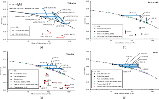
State diagram and CSL e–p′ idealisation: (a) TC; (b) θ = 0° (b = 0·5) α = 45°; (c) TE; and (d) HCSS
State diagram and CSL e–p′ idealisation: (a) TC; (b) θ = 0° (b = 0·5) α = 45°; (c) TE; and (d) HCSS
The CSL e–p′ idealisation shown in Fig. 8 was inferred from the LMT tests carried out under TC loading (Fanni et al. (2023) and the present study) using the power-law equation proposed by Li & Wang (1998). The parameters of this idealisation are presented in Fig. 8 and in equation (4). The critical state points inferred by Reid et al. (2022b, 2023) on the same material are included in Fig. 8, as reference states from previously published data from standard triaxial testing.
The uniqueness of the CSL e–p′ with respect to θ is investigated by comparing the end-of-test states of tests carried out under various stress paths against the CSL e–p′ idealisation inferred from TC loading. The results (TC, TE, θ = 0°, α = 45° and HCSS) indicate that, within a reasonable tolerance typical of element testing, the CSL e–p′ of the tailings is independent of stress path (i.e. isotropic or anisotropic) and θ, as all tests tend to a unique CSL e–p′. The maximum deviation from the idealised CSL e–p′ is approximately −0·015, but in general is within ±0·005. This range is well within typical experimental errors reported in the literature from CSL e–p′ characterisation when using only the TC testing, for example, Reid et al. (2021).
Most of the LMT tests clearly exhibited a typical critical state condition, characterised by and approximately zero (Figs. 6 and 7), except the θ = 0°, α = 45° and TE drained tests. Specifically, the θ = 0°, α = 45° drained tests show that εv increased while q remained approximately steady, whereas the TE drained tests indicate that q decreased while εv increased. The implication of these results on the inference of the CSL e–p′ is discussed below.
Examination of photographs of the θ = 0°, α = 45° and TE drained tests specimens (Fig. 9) indicates the presence of shear localisation. Although the undrained TE tests show a typical critical state condition, examination of the specimens during shearing clearly shows the presence of localisation characterised by a distinct horizontal shear plane within the specimen (Fig. 9(a)). The same shearing pattern was observed on the LMT TE drained specimens (Fig. 9(b)). The AD TE specimens presented two different localisation patterns – that is, within the specimen (Fig. 9(c)) and at the end of the specimen (bottom or top) (Fig. 9(d)). Photographs taken during shearing of a few LMT and AD TE specimens indicated that localisation typically occurred when the stress was at its maximum effective stress ratio ηmax. This observation is supported by the study carried out by Becker et al. (2022), which employed a photogrammetry method to correct stresses and states of TE specimens. The specimens were observed to maintain a right cylinder shape until reaching ηmax, suggesting that the lubricated platens may have made a positive contribution to the uniformity of shearing up to the onset of localisation, for example compared to the use of rough ends. Typically, ηmax mobilised in the LMT drained specimens after εq ≈ 8–10%, while in the undrained tests this occurred after εq ≈ 4–8%. The state diagram of TE includes the states at ηmax and the EoT states, which are clearly near or tending towards the CSL e–p′ inferred under TC loading. Despite the relatively small strain at which localisation may have initiated, this seems also to indicate that the CSL e–p′ under TE loading is located near the CSL e–p′ inferred from the TC tests. The authors note that of the studies previously mentioned, which focused on characterising the CSL e–p′ under TE loading (Been et al., 1991; Schnaid et al., 2013; Salvatore et al., 2017; Becker et al., 2022; Fotovvat & Sadrekarimi, 2022; Wagner et al., 2023), only Becker et al. and Salvatore et al. adopted a non-standard methodology to infer the critical state of TE specimens, namely, by way of photogrammetry (Becker et al., 2022) and X-ray tomography (Salvatore et al., 2017). The other studies adopted a standard interpretation methodology, as adopted in the present study.
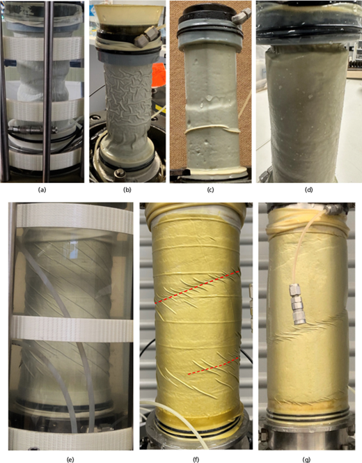
Typical specimen conditions at end of test: (a) TE LMT undrained; (b) TE LMT drained; (c), (d) TE AD drained; (e) θ = 0° (b = 0·5) α = 45° LMT drained; (f) θ = 0° (b = 0·5) α = 45° LMT undrained; and (g) θ = 0° (b = 0·5) α = 45° AD drained
Typical specimen conditions at end of test: (a) TE LMT undrained; (b) TE LMT drained; (c), (d) TE AD drained; (e) θ = 0° (b = 0·5) α = 45° LMT drained; (f) θ = 0° (b = 0·5) α = 45° LMT undrained; and (g) θ = 0° (b = 0·5) α = 45° AD drained
Regarding the θ = 0°, α = 45° tests, it can be noted that the undrained tests have reached a reasonable critical state condition and are tending to the CSL e–p′ inferred under TC loading. Moreover, based on visual observations the undrained specimens did not exhibit localisation (Fig. 9(e)). Therefore, the unclear EoT states noted in the drained tests could be explained by the presence of localisation (Fig. 9(f)) preventing these specimens from attaining a global critical state condition, while uniform shearing with diffuse distribution of pore pressure may have occurred in the undrained tests. The AD tests (Fig. 9(g)) presented localisation similar to the LMT drained tests, characterised by shear bands at an angle of approximately 72° from the vertical axis.
The data presented and discussed herein seem to further support that the CSL e–p′ of the tailings studied is independent of θ, and stress path in general, despite the limitation previously outlined resulting from the occurrence of localisation in some of the tests. This means that the CSL e–p′ could be determined using a standard axisymmetric TC device with this CSL e–p′ then applied to below-slope plane strain conditions that are most relevant to perimeter embankment stability.
Stress- and state-dilatancy
The stress- and state-dilatancy of the gold tailings were interpreted adopting the idealisation proposed by Jefferies & Shuttle (2011), wherein stress- and state-dilatancy relationships are defined according to the equations below.
where ηmax is the peak stress ratio; Dmin is the minimum dilatancy; N is the volumetric coupling parameter; and χ is the state-dilatancy coefficient (Jefferies & Shuttle, 2011). The stress- and state-dilatancy equations are linear locus defined at Dmin and at their corresponding state parameter (). The stress-dilatancy parameters were inferred by considering both loose and dense drained tests adopting the Shuttle & Jefferies (2016) and Bishop (1971) methods, respectively. Where required, M and N were manually adjusted to keep the stress-dilatancy asymptotic to the LMT stress-dilatancy line, according to the approach proposed by Shuttle & Jefferies (2016). The state-dilatancy was instead inferred by fitting the data to a linear trend passing through the origin (D = 0 and ψ = 0). The stress- and state-dilatancy inferred from the TC, θ = 0°, α = 45° and TE tests are presented in Fig. 10 with states summarised in Table 7.
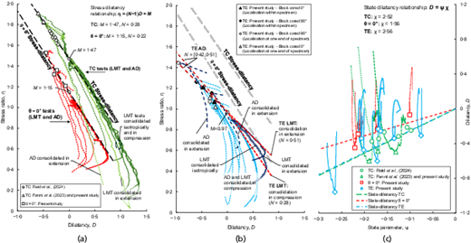
Stress-dilatancy: (a) TC and θ = 0° (b = 0·5) α = 45°; (b) TE. (c) State-dilatancy: TC, θ = 0° (b = 0·5) α = 45° and TE
Stress-dilatancy: (a) TC and θ = 0° (b = 0·5) α = 45°; (b) TE. (c) State-dilatancy: TC, θ = 0° (b = 0·5) α = 45° and TE
Stress- and state-dilatancy
| Test series | Test ID | Dmin | Ψ @ dmin | η @ dmin |
|---|---|---|---|---|
| TSHC TC | AD-01 | −0·49 | −0·171 | 1·82 |
| AD-02 | −0·60 | −0·190 | 1·91 | |
| TXC | AD-01 | −0·50 | −0·131 | 1·83 |
| TXC (Reid et al., 2024) | — | −0·25 | −0·098 | 1·65 |
| — | −0·32 | −0·126 | 1·68 | |
| — | −0·21 | −0·107 | 1·61 | |
| — | −0·38 | −0·184 | 1·74 | |
| — | −0·35 | −0·169 | 1·71 | |
| — | −0·27 | −0·157 | 1·68 | |
| θ = 0°, α = 45° | AD-01 | −0·07 | −0·101 | 1·21 |
| AD-02 | −0·24 | −0·172 | 1·36 | |
| AD-03 | −0·45 | −0·221 | 1·53 | |
| AD-04 | −0·29 | −0·214 | 1·32 | |
| TXE | AD-01 | −0·34 | −0·207 | 1·11 |
| AD-02 | −0·23 | −0·170 | 1·02 | |
| AD-03 | −0·26 | −0·165 | 1·07 | |
| AD-04 | −0·47 | −0·202 | 1·21 | |
| AD-05 | −0·60 | −0·172 | 1·26 | |
| AD-06 | −0·31 | −0·076 | 1·15 | |
| AD-07 | −0·96 | −0·265 | 1·45 | |
| AD-08 | −0·34 | −0·135 | 1·07 |
Dense AD and LMT tests were carried out with θ = 0°, α = 45°, consolidating the specimens at θ and α equal to the conditions of subsequent shearing. To investigate the effect of shear-stress anisotropy (initial and evolved) on the stress- and state-dilatancy of the tailings, TC and TE tests were sheared at the same stress condition of consolidation and by consolidating at θ and α opposite to its shearing direction (i.e. stress reversal). Further, TE on AD specimens were carried out on blocks trimmed at β = 0° and 90° to investigate the inherent anisotropy of AD specimens and its effects on stress- and state-dilatancy. The TE AD specimens that localised within the specimen typically showed higher ηmax than the specimens that localised at one end of the specimen, which might be explained by the occurrence of earlier localisation affecting the mobilisation of its peak strength. These data have not been used to infer stress- and state-dilatancy parameters.
The results of the AD tests indicate that the stress- and state-dilatancy may be approximated by linear relationships with locus following a unique trend independent of the fabric of AD (refer to AD TE tests on β = 0° and 90° blocks), initial shear stress and evolving anisotropy (refer to AD TC and TE tests sheared under stress-reversal conditions). The authors note that some numerical simulations have indicated that stress-dilatancy (e.g. Salimi & Lashkari, 2020; Wang et al., 2020) may depend on inherent anisotropy. Hence, the testing carried out in the present study may indicate that the fabric of dense AD could be not strongly anisotropic.
The drained TE AD tests suggest that the stress-dilatancy parameter N ranges between 0·42 and 0·51, with average 0·47. The results of the drained TE LMT tests indicate that the stress path influenced the stress-dilatancy of LMT specimens (Fig. 10(b)), wherein when testing was carried out with stress reversal (TE LMT-01/-02) the stress-dilatancy is non-linear, while it becomes linear when shearing is carried out at the same loading direction of consolidation (TE LMT-06) or isotropically (TE LMT-07). Excluding the initial elastic behaviour, the stress-dilatancy slope of TE LMT-06 is close to the stress-dilatancy inferred from TE AD, that is N = 0·51 and N = 0·47, respectively, while TE LMT-07 presents a stress-dilatancy slope in between TE LMT-06 and TE LMT-01/-02. Although smaller than TE, the stress reversal had some influence on the stress-dilatancy of LMT also under TC loading (Fig. 10(a)). The TC LMT tests sheared from isotropically (TSHC-TC LMT-01 and LMT-02) and anisotropically consolidated conditions (TXC LMT-03) exhibit similar stress-dilatancy slopes to AD, while the test sheared under stress reversal exhibits a different trend (TXC LMT-02). This might be attributed to a rearrangement of particles in the pre-shearing direction. The link between stress-reversal loading and dilatancy is particularly important in drained and undrained cyclic loading as it has been found to affect the cyclic response of materials (e.g. Dafalias & Manzari, 2004).
The TC data indicate MTC = 1·47 (critical friction angle ϕcr,TC = 36·2°), NTC = 0·28 and χTC = 2·52. The data reported by Reid et al. (2024) and Fanni et al. (2023) are in close agreement, which provides further confidence in the results produced in this study. The θ = 0° data suggest Mθ=0° = 1·15 (or ϕcr,θ=0°=41·7°), Nθ = 0° = 0·22 and χθ = 0° = 1·56. The results indicate that there is a variation of χ and N between the TC and θ = 0° loading conditions, while ϕcr,θ=0° > ϕcr,TC of approximately 6°. The variability of state-dilatancy parameters χ and N are within a plausible range based on the DEM results of Huang et al. (2014), as is the increase of ϕcr,θ = 0° compared to ϕcr,TC (e.g. Matsuoka & Nakai, 1974; Van Eekelen, 1980; Jefferies & Shuttle, 2002, 2011; Wanatowski, 2005; Huang et al., 2014). The TE data suggest MTE = 0·97 (or ϕcr,TE = 35·4°), NTE = 0·47 (ψ0 < 0) and χTE = 2·56. In this study, M in TE was estimated using Shuttle & Jefferies (2016) method, as the scatter in stress-dilatancy at Dmin was deemed sufficient to prevent the use of the Bishop method to accurately define M. Like the TC and θ = 0° tests, χ appears not to vary significantly with θ, an outcome consistent with the available literature (Jefferies & Shuttle, 2002, 2011; Huang et al., 2014). However, dense AD testing indicates that NTE > Nθ>0° and NTC. This outcome aligns with the results of Wagner et al. (2023) and Wang et al. (2020), but contradicts some available literature (e.g. Shuttle & Jefferies, 2002, 2011; Huang et al., 2014). The results also suggest that for the tailings studied the uniqueness of the CSL e–p′ in θ does not require an N independent of θ (as found by Wagner et al. (2023)) – indeed the data suggest the opposite, aligning with the DEM results of Wang et al. (2020). This means that to define the stress-dilatancy under generalised multiaxial stress conditions, constitutive models should also consider the evolution of N with θ.
The small difference between ϕcr,TE and ϕcr,TC of ≈0·8° seems plausible based on published data (e.g. Wu & Kolymbas, 1991; Shuttle & Jefferies, 2002; Huang et al., 2014; Jefferies & Been, 2016; Becker et al., 2022; Zhu et al., 2024) and acknowledging some of the limitations outlined due to localisation of TE specimens. Contrary to relevant literature and the present study, Fotovvat & Sadrekarimi (2022) reports for a sandy-gold tailings prepared adopting LMT, ϕcr,TE < ϕcr,TC of 20° for specimens isotropically consolidated and 9° for specimens anisotropically consolidated. It should be mentioned, however, that in Fotovvat and Sadrekarimi’s (2022) study most of the specimens exhibited phase transformation followed by dilation, hence the final state reported may have not reached a critical state condition, as outlined by the authors.
The yield surface at critical state inferred from the data are further interpreted in the π-plane in Fig. 11 by plotting the stress ratios (η = q/p′) at various values of θ. The figure includes the critical state surface based on typical M plotted against θ mathematical idealisations reported in the literature, indicating that Jefferies & Shuttle (2002, 2011) and Van Eekelen (1980) relationships fit the experimental results reasonably well.
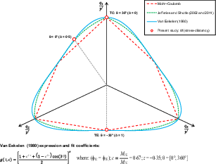
Yield surface at critical state in the π-plane: present study and typical relationships
Yield surface at critical state in the π-plane: present study and typical relationships
Undrained shear strength
The stress–strain behaviour of TC, TE, θ = 0°, α = 45° and HCSS tests are presented in Fig. 12 plots (a1), (b1) and (c1) as normalised deviatoric stress (q/) against εq, while the stress paths are shown in the same figure in the plots (a2), (b2) and (c2) as q/ against normalised mean effective stress (p′/). For clarity, the HCSS data are differentiated between tests carried out applying a static bias during consolidation from those without. As per Fig. 7, a negative sign has been assigned to the deviatoric stress in TE so that TE and TC tests can be distinguished in both stress–strain and stress-path plots. As previously indicated, all tests (except TSHC-TC LMT-05) contracted and strain-softened to a minimum strength, showing a behaviour typical of loose materials susceptible to liquefaction. In Fig. 13 the sign of q in TE loading is positive, consistent with the formulation presented in Table 1 and to allow comparison of the peak strengths obtained in the various tests. The data are sorted based on the pre-shearing stress parameter Kc calculated as the ratio between the minor (σ′3) and major (σ′1) principal stresses. The θ at yield (θy) of HCSS tests is reported for each test in Fig. 13(b). The yield states are summarised in Table 8. The results produced in the present study are complemented by the tests of Reid et al. (2021, 2022b) carried out on a similar tailings gradation at Kc = 0·5 and isotropic consolidation (Kc = 1·0).
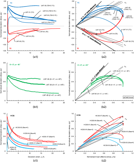
(a1), (a2) TC and TE; (b1), (b2) θ = 0° (b = 0·5) α = 45°; (c1), (c2) HCSS. (a1), (b1) and (c1) show undrained tests stress–strain (q/ plotted against εq); (a2), (b2) and (c2) show stress path (q/ plotted against p′/)
(a1), (a2) TC and TE; (b1), (b2) θ = 0° (b = 0·5) α = 45°; (c1), (c2) HCSS. (a1), (b1) and (c1) show undrained tests stress–strain (q/ plotted against εq); (a2), (b2) and (c2) show stress path (q/ plotted against p′/)
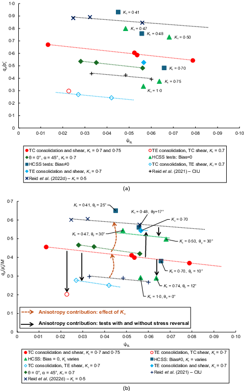
Instability undrained loading: (a) qp/ plotted against ψIL and (b) qp//M plotted against ψIL
Instability undrained loading: (a) qp/ plotted against ψIL and (b) qp//M plotted against ψIL
Undrained states at yield
| Test series | Test ID | Consolidated | Yield states | |||||
|---|---|---|---|---|---|---|---|---|
| Kc | θ: deg | M | ΨIL | qp/ | qp//M | ηIL | ||
| TSHC TC | LMT-03 | 0·75 | 30 | 1·47 | 0·079 | 0·54 | 0·37 | 0·77 |
| LMT-04 | 0·75 | 0·054 | 0·59 | 0·40 | 0·87 | |||
| LMT-05 | 0·70 | 0·013 | 0·67 | 0·46 | 0·99 | |||
| LMT-06 | 0·70 | 0·052 | 0·60 | 0·41 | 0·83 | |||
| TXC | LMT-01* | 0·70 | 0·023 | 0·30 | 0·20 | 0·81 | ||
| θ = 0°, α = 45° | LMT-04 | 0·71 | 0 | 1·15 | 0·028 | 0·54 | 0·47 | 0·73 |
| LMT-05 | 0·70 | 0·056 | 0·48 | 0·42 | 0·63 | |||
| LMT-06 | 0·68 | 0·035 | 0·53 | 0·46 | 0·71 | |||
| TXE | LMT-03* | 0·68 | −30 | 0·97 | 0·042 | 0·24 | 0·25 | 0·55 |
| LMT-04* | 0·70 | 0·027 | 0·27 | 0·28 | 0·62 | |||
| LMT-05 | 0·70 | 0·057 | 0·53 | 0·54 | 0·67 | |||
| HCSS | HCSS-01* | 0·47 | 30 | 1·47† | 0·048 | 0·80 | 0·54 | 0·80 |
| HCSS-02* | 0·74 | 12 | 1·30† | 0·064 | 0·38 | 0·29 | 0·59 | |
| HCSS-03* | 0·99 | 0 | 1·15† | 0·056 | 0·34 | 0·29 | 0·58 | |
| HCSS | HCSS-04 | 0·48 | 17 | 1·35† | 0·056 | 0·76 | 0·56 | 0·80 |
| HCSS-05 | 0·70 | 10 | 1·27† | 0·066 | 0·48 | 0·38 | 0·62 | |
| HCSS-06 | 0·50 | 30 | 1·47† | 0·068 | 0·73 | 0·50 | 0·73 | |
| HCSS-07 | 0·41 | 25 | 1·43† | 0·045 | 0·93 | 0·65 | 0·94 | |
*Stress-reversal tests
†Calculated using Van Eekelen relationship
The deviatoric stress at yield (qp/), represented by qp at the onset of strain-softening and undrained instability, is presented in Fig. 13(a) against ψ at the onset of undrained instability (ψIL) (e.g. Chu et al., 2003). The yield deviatoric stress normalised by M is presented in Fig. 13(b). The M used in the normalisation was calculated using the Van Eekelen (1980) relationship shown in Fig. 11 for the specific θ in the test. This normalisation was applied to investigate if yielding scales with θ in a similar manner as with M (refer to Fig. 11) and to investigate the effect of anisotropy. The yield surface at critical state may be assumed to represent an anisotropic independent yield surface, as there is evidence that at critical state even materials with strong anisotropy produce a unique critical state particles orientation (e.g. Li & Dafalias, 2012 ; Salimi & Lashkari, 2020). Hence, the shape of this surface is adopted as a reference locus to assess the effect of anisotropy on the yield undrained strength. Therefore, any deviation from the normalised strength based on Fig. 11 is assumed to be due to anisotropy. Based on this assumption, the effect of anisotropy is shown in Fig. 13(b) as arrows indicating negative (pointing downwards) or positive (pointing upwards) strength contributions.
Figure 13 indicates that qp/ does not show a strong dependency on ψIL. This is likely to be the result of LMT samples being prepared in a very loose state, as if specimens had been prepared to denser states, the influence of ψIL would have been likely more pronounced, in particular when approaching states near the contractive/dilative boundary (typically at ψ0 ≈ −0·05 to −0·10 (Jefferies & Been, 2016)). Alternatively, the influence of Kc on qp/ is noted in Fig. 13, wherein the yield strength is shown to increase as Kc (or ηc) increases (e.g. TC at Kc = 0·5 as opposed to TC at Kc = 0·70–0·75), consistent with the testing of Fotovvat & Sadrekarimi (2022). This may be explained by the contribution of the initial shear-stress anisotropy which, through a rearrangement of particles in the pre-shearing direction, may have caused a shift of the yield locus towards the direction of loading (e.g. Imam et al., 2002). The contribution of θ and α on the yield strength is evident comparing the qp/ of TC with tests carried out under other stress conditions, wherein for similar Kc, TC shows systematically the greatest strengths (Fig. 13(a)).
By comparing the HCSS with and without bias, it is evident that consolidation carried out under α > 0° and θ < 30° (stress states more typical of below-slope conditions) has a positive effect on the yield strength of LMT (refer to θ = 0°, α = 45° and HCSS with bias tests). Indeed, the yield strength increases with the static stress, although at the expense of a more brittle behaviour (Fig. 12). This indicates that evolving anisotropy may have induced a rearrangement of particles in the direction of loading, leading to a shift and/or rotation of the yield locus towards the direction of loading. The results are consistent with the observations of Jardine & Smith (1991) on the effect of bias on the strength of foundation soils during multi-stage embankment construction, a construction method typically adopted in TSFs.
For testing carried out under TC, θ = 0°, α = 45° and HCSS with bias under anisotropic consolidation without stress reversal, the normalisation by M (Fig. 13(b)) produced an almost unique function independent of θ and α. This suggests that for these tests the undrained yield surface scales with θ in a similar manner as M (Fig. 11), such that under these conditions the behaviour at yield could be simplified by scaling the yield surface based on TC strength, but without applying a shift and/or rotation of the yield surface. However, this is not observed for the TE carried out without stress reversal, wherein qp/ is close to the TC trendline and plots above it once scaled by M – a behaviour similar to the tests reported by Fotovvat & Sadrekarimi (2022). A similar conclusion can be deduced for the tests sheared under stress reversal (TE, TC and HCSS without bias). However, in these tests, the yield strength remains below the strength envelope for TC, θ = 0°, α = 45° and HCSS with bias, even following scaling by M. This indicates that the initial shear-stress anisotropy has a positive contribution on the yield strength when shearing is carried out without stress reversal, but negative when sheared with stress reversal. Under this condition scaling of the yield surface based on TC strength would not be sufficient, and a shift and/or rotation would be also required.
Similarly to some of the anisotropically consolidated tests, the results of the isotropically consolidated tests sheared under TC and HCSS without bias indicate that the normalisation by M has produced an almost unique function, hence following in θ space the same shape of the yield surface at critical state. This indicates that the fabric of LMT may not be strongly anisotropic, a conclusion consistent with the particle arrangement analysis of MT carried out by Yang et al. (2008) on sand based on scanning electron microscopy testing.
CONCLUSIONS
This study has presented the results of testing carried out on LMT and dense AD specimens of sandy silt gold tailings sheared under various stress paths. The work focused on examining the effect of θ on the CSL e–p′ and on the stress- and state-dilatancy, and the effect of various stress paths and anisotropy on the yield undrained shear strength of LMT tailings specimens.
The results of the tests indicate that the CSL e–p′ of the tailings is independent of θ, as well as the stress path (i.e. isotropic or anisotropic) at consolidation. This means that the CSL e–p′ of the tailings could be determined by way of standard, isotropically consolidated triaxial testing.
Examination of the tailings stress- and state-dilatancy from dense AD specimens indicates that the stress- and state-dilatancy does not depend on anisotropy. Testing carried out with and without stress reversal indicates that when the tailings are prepared loose using moist tamping, the stress-dilatancy depends on the stress path, a behaviour attributed to stress anisotropy. The trend between M (slope of CSL in q–p′ plane) and θ can be approximated by adopting typical mathematical relationships available in the literature (i.e. Van Eekelen, 1980; Jefferies & Shuttle, 2002, 2011). The ϕcr measured in TC, θ = 0° and TE was approximately 36°, 42° and 35°, respectively. The state-dilatancy coefficient χ was found to vary slightly with θ, while stress-dilatancy coefficient N was found to be similar between TC and θ = 0°, but under TE it was found that NTE > Nθ>0° and NTC.
The undrained yield strength of tailings specimens subjected to undrained shearing following various stress paths (TC, TE, θ = 0°, α = 45°, HCSS with and without bias) indicates that the strength does not strongly depend on ψ, while it shows a strong dependency on the stress conditions adopted at consolidation. It was found that the initial shear stress and evolving anisotropy had a significant effect on the yield strength of the tailings. Specifically, the data indicate that the initial shear-stress anisotropy has a positive contribution to the yield strength when shearing is carried out without stress reversal but negative when sheared under stress reversal. Furthermore, the data indicate that when consolidation is carried out under typical below-slope stress conditions (e.g. α > 0° and θ < 30°, HCSS tests with bias) the yield strength of LMT increases with increasing static stresses. This suggests that initial shear stress and evolving anisotropy may have induced a rearrangement of particles in the direction of loading causing a shift and/or rotation of the yield surface towards the same direction of loading.
DATA AVAILABILITY STATEMENT
Data generated during this study are available in the OFS repository, in accordance with data retention policies, at this link: https://osf.io/sb2nf/?view_only=4614648259f446d4a61f83fe8360cedd.
MATERIAL AVAILABILITY STATEMENT
Material used for testing in this study are available from the corresponding author upon reasonable request.
REFERENCES
Discussion on this paper closes 1 May 2026; for further details see p. ii.

