Factor of safety of pile-stabilised slopes: an algorithm incorporating soil-arching effect Open Access

D

diameter of stabilising piles

E

modulus of elasticity

E_i

normal inter-slice force

F_s

Factor of safety of slope

H

depth of the pile above the slip surface

K_an

new coefficient of lateral earth pressure incorporating soil arching

K_c

horizontal seismic coefficient

M_s

additional moment due to installation of the piles

$Ni′$

effective normal force on the base

P

lateral resistance offered by the pile per unit depth

P_i

resultant lateral force acting on post-arching zone

P_o

resultant reaction on pre-arching zone

P_r

resultant lateral force on pile

Q_i

external force on (i ^th) slice

$Si′$

mobilized shear resistance on the base of a slice

U

resultant pore water force

W_i

self-weight of i ^th slice

X

inter-slice shear force

b_i

width of i ^th slice

c

cohesion of the soil

h_i

height of i ^th slice

l_a

length of horizontal arching zone

n

ratio of centre-to-centre spacing and pile diameter

s

centre-to-centre spacing between piles

u

average pore water pressure

α_i

base inclination of i ^th slice

β

angle of soil slope with horizontal

γ

unit weight of soil

Λ

spacing coefficient

λ

scale factor

λ_m

proposed scale factor

μ

Poisson’s ratio

φ

angle of internal friction of soil

Ψ

angle of dilatancy of soil

σ_i

radial stress on the inner arch of horizontal arching zone

$σ¯v$

average vertical stress on a differential element dz

The stability of slopes is one of the fundamental problems in geotechnical engineering as their delicate balance is often disrupted by natural or man-made causes. Furthermore, the increasing demand for engineered cut-and-fills, construction near or on slopes and so on, has increased the need to understand the mechanism of slope failure and develop techniques to stabilise the slopes. Stability of slopes depends on the balance between a driving force that causes failure and a resisting force that is developed against it. All the slope stabilisation methods basically try to reduce the driving force or increase the resisting force or both. One of the operative techniques employed for stabilisation of slopes and prevention of excessive soil movement is using stabilising piles in row(s) (Ashour and Ardalan, 2012; Ausilio et al., 2001; Cai and Ugai, 2000; Hassiotis et al., 1997; Ito and Matsui, 1975; Kourkoulis et al. 2011a; Liang et al. 2014; Lirer, 2012; Neeraj and Thiyyakkandi, 2020). In practice, the piles are installed well beyond the potential slip surface to the firm ground beneath it to arrest the possible sliding of unstable soil mass. The piles act as a cantilever beam that takes the lateral forces due to the sliding soil mass and transfer them to the stable ground underneath it (Ellis et al., 2010; Liang and Zeng, 2002). This additional resistance provided by the piles stabilises the slope, thus improving its factor of safety (F_s) against failure. The computation of F_s of pile-stabilised slopes is conventionally done by extending the methods used for analysis of normal slopes to incorporate the additional forces generated due to installation of piles.

The stability of normal slopes can be analysed by numerous methods such as the limit analysis method, variational calculus method, strength reduction method, limit equilibrium method and so on (Atarigaya, 2016). The need for considering different forces (e.g. body force, pore water pressure, etc.) and diverse soil types in the stability analysis of slopes invalidates the use of conventional methods in the mechanics of continua, and consequently, the limit equilibrium method is commonly adopted (Morgenstern and Price, 1965). One of the earliest known and most widely used concepts of limit equilibrium is explained through method of slices owing to the ease of computation (Ahmed, 2017; Atarigaya, 2016; Duncan, 1996; Firat, 2009; Hassiotis et al., 1997; Tsuchida and Athapaththu 2014; Zhu et al., 2005). The analysis is done by dividing the slope into a number of slices to find out the factor of safety of the slope. Various methods commonly used for formulation of F_s in the method of slices are the Fellenius Swedish circle or ordinary method, Bishop’s simplified method, Janbu method, Spencer method and Morgenstern–Price method. All these limit equilibrium methods use the Mohr–Coulomb criterion to determine the shear strength of soil along the failure surface. The choice of method depends largely on the type of soil and the required accuracy of the work. The most widely used method for the analysis of a generalised slip surface is the Morgenstern–Price method (Ahmed, 2017; Atarigaya, 2016; Firat, 2009; Griffiths and Lane, 1999). This method considers both moment and force equilibriums to produce a non-linear indeterminate equation for F_s. The equation is made determinate by assuming a function that relates the inter-slice shear force to inter-slice normal force.

The methods mentioned above are applicable for the case of normal slopes that are not stabilised by piles. At present, the study of pile-stabilised slopes is generally carried out by extending these conventional methods (Di Laora et al., 2017; Firat, 2009; 1995; Jeong et al., 2003; Kourkoulis et al., 2011; Lee et al., 1995, Summersgill et al., 2018). The resistance offered by the piles is added as an additional term in the formulation of F_s, which does not account for the propagation of reactive force through soil. A major issue in this approach is that the critical slip surface considered is the same as that of non-stabilised soil slopes (Firat, 2009; Kourkoulis et al., 2011; Lee et al., 1995; Summersgill et al., 2018). However, in reality, due to the introduction of piles, the critical slip surface changes and this modified surface needs to be considered while computing the F_s. Also, the conventional methods fail to incorporate the effect of location of piles along the slopes (Hassiotis et al., 1997; Lirer, 2012; Neeraj, 2019; Summersgill et al., 2018). In the present study, the Morgenstern–Price method is modified using the method of slices to adopt for the analysis of pile-stabilised slopes such that the cumulative effect of lateral resistance offered by the pile on each slice is accounted for. An algorithm is developed to compute the F_s of the pile-stabilised slope considering the modified critical slip surface. The proposed algorithm can be easily switched to use for both normal slopes and pile stabilised slopes. Finite-element modelling of both normal and pile-stabilised slopes was carried out and the obtained F_s values were used to validate the proposed algorithm. The variation of F_s with the location of the pile along the slope was studied. Subsequently, a simple technique to determine the optimal pile location is explained.

The F_s computation using the proposed algorithm requires accurate determination of lateral resistance offered by the stabilising piles. Due to the resistance from the pile and differential movement of soil in between the piles, the soil-arching effect plays a key role in the load-transfer mechanism of pile-stabilised slopes. Several methods have been proposed in the past to estimate the lateral resistance offered by the row of piles incorporating the effect of soil arching. One of the pioneering attempts to model the soil-arching effect due to the differential lateral deformation of soil between the piles in the horizontal direction (termed as ‘squeezing effect’) was by Ito and Matsui (1975). However, the method does not consider the rotation of principal stresses due to soil arching. Most of the methods developed afterward have adopted or modified the ‘squeezing concept’ considered by Ito and Matsui (1975) (Fırat 2009; Harrop-Williams, 1989; He et al., 2015a; He et al., 2015b; Li and Wei, 2018; Song et al., 2012; Won et al., 2005). As the soil in front of the piles deforms vertically, the lateral earth pressure distribution adjacent to the stabilising piles will become non-linear due to the vertical arching. Adopting the formulation of Ito and Matsui (1975), He et al. (2015a) presented an analytical method to determine the non-linear pile resistance in sandy slopes incorporating vertical arching. The method was extended by He et al. (2015b) for c−φ soil; however, it does not account for the effect of slope angle. In reality, both horizontal and vertical arching need to be considered to determine the lateral resistance offered by the stabilising piles. Recently, Neeraj and Thiyyakkandi (2020) presented a general method (for c−φ soil) to determine the lateral pile resistance incorporating the effect of soil arching in horizontal and vertical directions. The method also considers the effect of slope angle (β) in the design. In this work, the method of Neeraj and Thiyyakkandi (2020) is extended to model the gradual propagation of pile resistance as explained in subsequent sections.

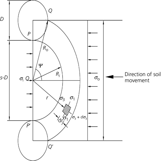
An analytical method to obtain the lateral resistance offered by the row of piles considering the effect of soil arching in both the horizontal and vertical direction was proposed by Neeraj and Thiyyakkandi (2020). The stress state of the soil-arching zone in the horizontal direction is presented in Figure 1. The resistance offered by the stabilising piles is given by:

Where, Λ is the spacing coefficient given by, $Λ=[(n2+1n−1)N−1−1]n$⁠; here n is the ratio of pile spacing to the diameter of the piles (n = s/D) and N = tan² 45 + φ/2. The term c represents the cohesion of the soil, and φ the angle of internal friction. The stress, σ_i, acting along the central plane of pile row is a function of average vertical stress (⁠$σ¯v$⁠) as given by:

Where:

$Kan=cos(θw+ξ)cosβcos(β+ξ)[3(Ncos2θw+sin2θw)3N−(N−1)cos2θw]T=2cN[cos2θw(3(Ncos2θw+sin2θw))3N−(N−1)cos2θw−sin2θw]$

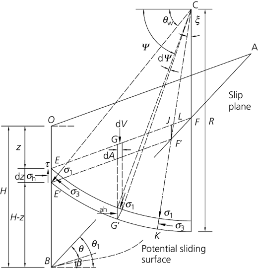
The stress state including the direction of the major and minor principal stresses after vertical arching in the active plastic zone behind the row of piles is shown in Figure 2. A differential element EFF′E′ is assumed to take a circular shape due to vertical arching caused by the shear resistance developed along the vertical plane OB. An intricate analysis considering the force equilibrium of the differential element results in the formulation of an expression for average vertical stress, $σ¯v$⁠, given by (Figure 2):

Where:

$C1=(Kantanφ−Kantanβ+m)sinθcosθ1;m=KanNcos2θ+sin2θsinξcosβcos(ξ+β)$

$C2=(Ttanφ−Kantanβ+t)sinθcosθ1;t=c+(T+2csin2θ/NNcos2θ+sin2θ)sinξcosβcos(ξ+β)$

where, θ is the angle between the slip plane and the slope surface; θ₁ is the angle between the slip plane and the horizontal; β is the slope angle; and ξ is the angle between the major principal stress and vertical at point where the differential element dz intersects the slip plane; which are given by:

$ξ=π4+φ2−θ1$⁠; $θ=12(φ−β+cos−1sinβsinφ)$⁠; and $θ1=12(φ+β+cos−1sinβsinφ)$

The average vertical stress (⁠$σ¯v$⁠) varies non-linearly with depth of the pile due to the vertical arching of soil. The detailed derivation of Equation 3 is presented in Appendix A.

The resultant force (P_r) offered by the row of piles can be obtained by integrating Equation 1 with respect to the depth of the pile:

Further details about the derivations of Equations 1–4 can be found in the paper by Neeraj and Thiyyakkandi (2020). The analytical method described above is adopted to obtain the lateral resistance offered by piles. The method is further extended in this work to be used in the determination of F_S of pile-stabilised slopes as explained in the following section.

As mentioned in the Introduction, the Morgenstern–Price method is used in this study to analyse slope stability. According to Morgenstern and Price (1965), the inter-slice shear forces (X_i) can be related to inter-slice normal forces (E_i) by a predefined function f(x) as given in Equation 5. The direction of inter-slice forces varies according to the assumed function.

Where:

f(x) = inter-slice function that varies continuously along the slip surface

λ = scale factor for the assumed function

Theoretically, the force function f(x) can take any form. However, the nature of soil imposes certain range of functions that can be rationally used for all practical purposes (Morgenstern and Price, 1965). Commonly used functions are constant, half-sine, trapezoidal, user-defined, and so on. In this analysis, f(x) is assumed as a half-sine function. An algorithm, based on the Morgenstern–Price method, developed by Zhu et al. (2005) to determine the F_s for soil slopes that are not stabilised by piles is modified to incorporate the effects of additional reactive forces generated due to the introduction of stabilising piles. The solution is developed such that both moment equilibrium and force equilibrium are satisfied.

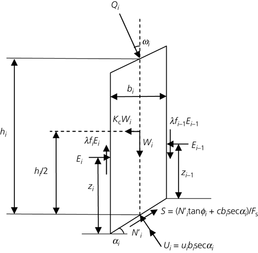
Figure 3 shows the free-body diagram of a typical slice (i^th) with height h_i, width b_i and base inclination α_i. The slice is subjected to a self-weight W_i and seismic force K_cW_i, where K_c is the horizontal seismic coefficient, with external force Q_i acting at an angle ω_i to the vertical, resultant pore water force U_i = u_ib_isec α_i, where u_i is the average pore water pressure, effective normal force on the base $Ni′$ and mobilized shear resistance $Si=(Ni'tanφi'+ci'bisecαi)/Fs$⁠, where $φi′$ is the effective angle of internal friction, $ci′$ is the cohesion along the base of the slice and F_s is the factor of safety for the slip surface. F_s is assumed to be constant along a slip surface. The soil slice is also subjected to normal inter-slice forces E_i and E_i−1 on the left and right boundaries of the slice at a height z_i and z_i−1 from the bottom, respectively. Inter-slice shear forces are calculated using Equation 5.

The equation for F_s developed by Zhu et al. (2005) based on the Morgenstern–Price method for soil slopes that are not stabilised by piles is as given below.

Where:

In reality, R_i is sum of the components of all the forces acting on a slice contributing to the resisting force except the inter-slice normal forces, and T_i is sum of all the forces that contribute to the driving force that cause instability. As the F_s term exists on both sides of Equation 6, an iterative procedure has to be adopted to solve for F_s, with an assumed value in the first trial.

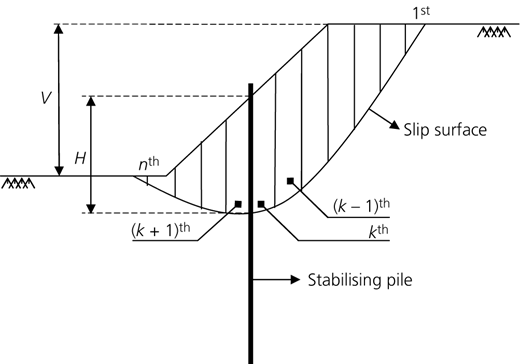
To incorporate the influence of stabilising piles in the safety analysis of slopes, a pile-stabilised slope as shown in Figure 4 with pile located at the k^th slice is considered. The slope is demarcated into three zones, namely, the pre-arching zone, the arching zone and the post-arching zone. The region k in Figure 4 represents the arching zone. The (k − 1)^th and (k + 1)^th slices are located to the right and left of the arching zone, respectively.

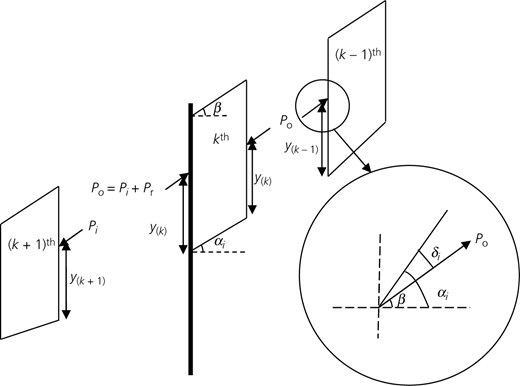
Figure 5 shows an enlarged view of the arching zone and the adjacent slices with the additional forces that occurs due to the introduction of piles. It should be noted that all the forces shown in Figure 3 also act on these slices, although they are omitted in Figure 5 to improve clarity. The width of the k^th slice is assumed to be the length of horizontal arching zone (Figure 1), given by:

From the analytical solutions presented in the previous section, the resultant pile force P_r is the difference between the force P_o acting on the right edge of arching zone and the force P_i acting on the left edge of the arching zone (Neeraj, 2019).

The points of application of lateral thrusts P_o and P_i are given by y_k−1 = M_o/P_o, and y_k+1 = M_i/P_i, respectively, where M_o and M_i are corresponding moments along the slip surface. The detailed derivation of resultant forces (P_o and P_i) and moments (M_o and M_i) in the pre-arching and post-arching zones and the points of action (y_k−1 and y_k+1) is presented in Appendix B.

The forces P_o and P_i are considered as external forces acting on the corresponding slices. They are resolved in the normal and tangential direction with respect to base of each slice and incorporated in R_i and T_i of corresponding slices as shown in Equations 17–20.

where, δ = |α − β| is the inclination of resultant additional force (P_o or P_i) with reference to the respective slice base as shown in Figure 5. Since the k^th slice has equal forces acting from both sides (P_i + P_r = P_o¸ on the right edge and P_o on the left edge), R_k and T_k remain unchanged. However, the moment equilibrium of the slice is influenced by these forces as their lines of action differ. Specifically, an additional moment M_a is generated as given in Equation 21.

Since the present method does not consider the pile’s contribution as an additional component explicitly, the equation for F_s (Equation 6) remains the same. However, the scale factor λ needs to be modified to incorporate the additional moment M_a (Equation 21) developed on k^th slice as follows,

The modified scale factor, λ_m, has to be used in Equations 7, 10 and 11 for F_s calculation.

As indicated earlier, an iterative procedure is required to solve for the factor of safety. An iterative algorithm was developed for determining the critical slip surface and corresponding F_s for a given pile-stabilised slope. The steps involved in the iteration are as follows.

1. Input the slope geometry (height, V and slope angle, β); soil properties (γ, c and φ); and pile parameters (D and S).

2. Divide the whole slope into a number of slices.

3. Input pile location (k) and compute the length of the soil-arching zone (l_a).

4. Choose an arbitrary slip surface and input entry and exit points.

5. Calculate the resultant forces acting on k^th, (k − 1)^th and (k + 1)^th slices (P_r, P_o and P_i) and the additional moment (M_a) developed due to the introduction of the piles, using Equations 4, 15, 16, and 21, respectively.

6. Calculate R_i and T_i for all the slices using Equations 12 and 13, respectively.

7. Modify R_i and T_i for (k − 1)^th slice and (k + 1 )^th slice using Equations 17–20.

8. Define the inter-slice function f(x). A half-sine function is assumed here:

   $f(x)=sin[π(x−xminxmax−xmin)]$

   where, x_max and x_min are abscissa of entry and exit points of the failure surface, respectively, and x denotes the abscissa of midpoint of each slice.

9. Assume an initial value for F_s and λ_m. The number of iterations required depends on the initial values assumed. However, the final values of F_s and λ_m do not vary with the assumed initial values. An effective transfer of inter-slice normal force requires the assumed F_s to satisfy Equation 7 (Zhu et al., 2005). In general, for the first iteration, it can be assumed that F_s = 1 and λ_m = 0.

10. Calculate Ψ_i and Φ_i and for all slices using Equations 7 and 11.

11. Calculate F_s using Equation 6.

12. With F_s obtained from step 11 and the assumed value of λ_m, repeat steps 10 and 11 once more for the improved values of Φ_i, Ψ_i and F_s.

13. Calculate E_i using Equation 9.

14. Calculate λ_m using Equation 22.

15. With the updated values of F_s and λ_m, repeat steps 10–15 until the difference in the values of F_s and λ_m for two consecutive iterations fall below the tolerances t₁ and t₂, respectively. A tolerance of 0.001 was considered for both cases in this analysis.

16. Store the F_s value for the chosen slip surface.

17. Choose a different slip surface and return to step 4. Repeat up to step 17 for all the possible slip surfaces.

18. Find the minimum of all the F_s values obtained in step 17 to obtain the factor of safety and the critical slip surface of the pile-stabilised slope.

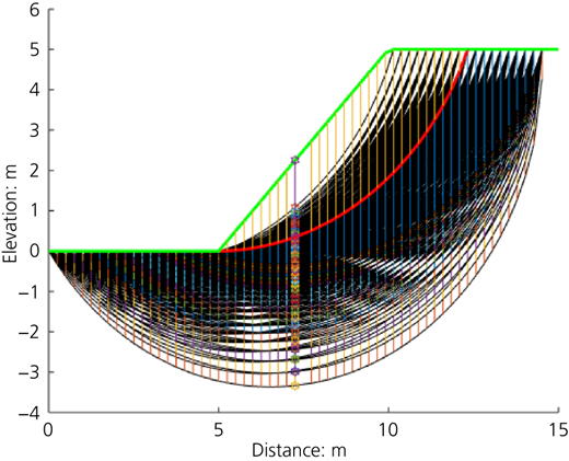
The above algorithm was coded in Matlab software (R2020b). The algorithm can also be used to obtain the F_s of soil slopes that are not stabilised by piles if R_i and T_i are calculated using Equations 12 and 13, respectively, for all slices and the scale factor (λ) is determined using Equation 8. Also, for the no-pile condition, the division of the slope into three zones is not needed. Figure 6 shows the typical output plot with various slip surfaces considered and the failure surface corresponding to the minimum F_s, for a particular pile position and slope angle. The abscissa and ordinate represent the respective horizontal and vertical dimensions of the model considered in the analysis. The critical slip surface is represented by red colour and the green lines represent the ground surface. The line with star marks at either ends denotes the location of the pile.

Factor of safety values for soil slopes with and without piles obtained from the proposed algorithm were compared with that determined using finite element modelling. Slopes without pile were modelled both in Plaxis 3D software and the Slope/W program of the GeoStudio software package. The Slope/W program is widely used to obtain the factor of safety of normal soil slopes. Pile-stabilised slopes were simulated only in Plaxis 3D as Slope/W program is a two-dimensional modelling tool. A soil slope having a height of 5 m and slope angle (β) of 26.6° (1V:2H) was modelled using various soil conditions and pile parameters as shown in Table 1. Two different soil conditions represented as Soil A (sand) and Soil B (c−φ soil) were chosen for the analyses. In the case of the pile-stabilised slope, a row of 0.3 m and 1 m dia. piles at a spacing of three times the diameter was considered. Modelling of slope sections with different number of piles was carried out and the results were essentially the same. The model presented here was the one with nine piles.

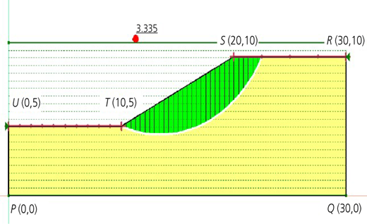
Figure 7 displays the slope model constructed in limit equilibrium slope stability mode of Slope/W. Morgenstern–Price analysis type was selected with a half-sine side function as adopted in the proposed algorithm. The soil was characterised as Mohr–Coulomb material and the phreatic line was assumed to be at a greater depth below base of the model. The potential slip surfaces for analysis were defined using entry and exit points with the specified ‘radius tangential lines’ intrinsic option available in the program.

In case of Plaxis 3D analysis, three-dimensional (3D) models of soil slope (and piles) were generated using 10-nodded tetrahedral elements. The built-in ‘soil and interface’ material type was selected to model soil and piles. The soil was modelled as Mohr–Coulomb material. The piles were modelled as concrete piles using the linear-elastic material model. The boundary condition at all the vertical surfaces was set to normally fixed. The horizontal surface at the base was fully restrained. The slope surface and the horizontal surfaces at the top were set to free. Sufficient depth of soil was provided below the pile tip so that the influence of boundary was negligible. The effect of construction sequence and pile installation were not considered in the present analysis. The soil mass and the piles were activated in the initial phase and a K_o calculation type was chosen. A null plastic analysis in phase 2 of the staged construction loading type was carried out to activate the gravity loads due to the soil mass and the row of piles. The plastic analysis was followed by the inbuilt safety analysis with updated mesh to determine the factor of safety of pile-stabilised slopes. The principle of strength reduction was used to obtain the factor of safety. Factor of safety is defined as the ratio of maximum available shear strength to minimum shear strength required for equilibrium. The standard Coulomb condition is introduced to strength reduction method to obtain Equation 23 for factor of safety (Brinkgreve et al., 2018).

where, c and φ are input strength parameters which are reduced to c_r and φ_r, the minimum required strength parameters, and σ_n is the normal stress component. In the strength reduction approach of Plaxis 3D, both c and φ are reduced by a common multiplier ∑M_sf as given in Equation 24. This parameter is incrementally increased till failure and the value of M_sf at failure is reported as factor of safety (Brinkgreve et al., 2018).

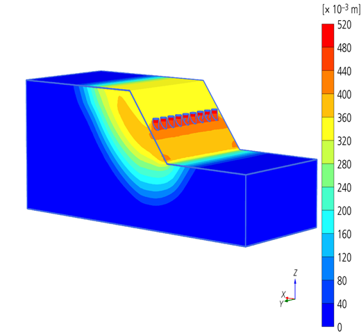
Figure 8 shows the total deformation contour obtained from the safety analysis of pile-stabilised slope in Plaxis 3D. Table 2 summarises the F_s values for slopes without piles for different soil types obtained from the proposed algorithm and finite-element modelling.

The comparison of F_s values of pile-stabilised slopes for the case of 0.3 and 1 m dia. piles, estimated using Plaxis 3D, and the developed algorithm are presented in Table 3. The F_s values for the same slope and pile-dimensions, when computed by taking the pile contribution explicitly as an additional term, are also presented in Table 3. This was obtained by adding P (Equation 1) to the numerator of equation for F_s (Equation 6) wherein R_i, t_i and λ were obtained using Equations 12, 13 and 8, respectively, as discussed previously for the case of non-stabilised slopes.

As is evident from the tables, the factor of safety values for both normal and stabilised slopes predicted using the proposed method were in close agreement with that obtained from the numerical analyses. This implies that the proposed algorithm can be used to compute the F_s quickly, unlike the finite-element packages which require a significant amount of time to generate a model and calculate the results. It can be observed from Table 3 that considering the resistance offered by piles as an additional term in the equation for F_s, as conventionally done in practice, leads to an over-prediction. The ‘additional term’ method also fails to capture the effect of pile location. In reality, the F_s varies with the location of piles, as discussed in next section.

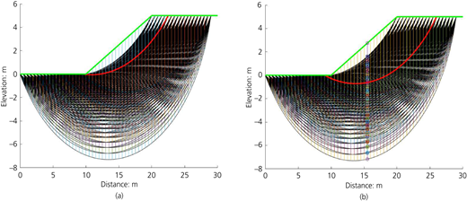
The installation of piles in a slope modifies its critical slip surface. The existing practices do not consider the change in critical slip surface and compute the factor of safety corresponding to the same slip surface as that of un-stabilised slopes. The proposed algorithm identifies the new critical slip surface formed due to the introduction of piles and computes the F_s corresponding to the new surface. To demonstrate the modification of slip surface due to the introduction of stabilising piles, the analyses were carried out for without and with stabilising piles cases using the proposed algorithm. Piles having a diameter of 1 m spaced at a centre-to-centre distance, n = 3, in a typical c−φ soil slope with c = 30 kN/m², φ = 20°, unit weight, γ = 20 kN/m³, and slope angle β = 26.5 (2H:1V) were considered for the analyses. When all other factors are kept constant, the variation in the critical slip surfaces for the case of without and with stabilising piles obtained using the proposed algorithm is given in Figures 9(a) and 9(b), respectively. The colour codes adopted for Figure 6 are applicable to Figure 9 as well.

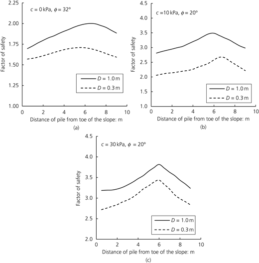
The factor of safety of pile-stabilised slopes is influenced by the location of the pile. Currently, the determination of optimal location of pile (OPL) is a time-consuming task which involves multiple finite-element modelling iterations, consuming considerable amounts of time. A new a straightforward technique to determine the OPL is presented in this work. The distance of the pile from the toe of the slope can be easily taken as an additional variable in the proposed algorithm presented in the previous section and the F_s value corresponding to each pile location can be computed. Three typical scenarios, (i) c = 0 kN/m², φ = 32°, (ii) c = 10 kN/m², φ = 20° and (iii) c = 30 kN/m², φ = 20°, were considered. A pile-stabilised slope installed with (i) D = 0.3 m and (ii) D = 1 m piles, spaced at a center-to-center distance, n = 3, and a slope angle β = 26.5° (2H:1V) was adopted. The unit weight of soil was assumed as 20 kN/m³. The total length of the base of the slope was adopted as 10 m. The variation of F_s with the location of pile for cases (i)–(iii) is presented in Figure 10(a)–(c).

The optimal location of pile obtained using the proposed method is in accordance with the results of past finite-element analyses found in literature. Hassiotis et al. (1997) suggested that the piles installed between the middle and the crest of the slope are most effective. In case of homogenous purely cohesive soil, Lee et al. (1995) showed that the most effective position of piles is close to the crest of the slope. The finite-element analysis presented in the paper by Cai and Ugai (2000) indicates that the piles located at the middle of the slope provide the highest factor of safety. Ausilio et al. (2001) also suggest placing the piles in the upper-middle portion of the slope for efficient stabilisation. As can be observed from Figure 10, the F_s values initially increase with the distance of pile from the toe of the slopes, reach a peak value and then decrease as the piles move further away from the toe. In case of sandy soil, the maximum factor of safety is obtained when the piles are located around the mid-slope. On the other hand, as the soil becomes cohesive, the maximum F_s value is found to occur at a pile location above the mid-slope. However, the location of pile corresponding to the peak value of F_s can not be readily called the OPL as it is also influenced by various other factors, for example, the access to the slope, space for construction and so on. Nevertheless, the proposed algorithm can be easily used to obtain the variation of factor of safety with location of pile, which in turn can be used by engineers to choose the location based on other field constraints.

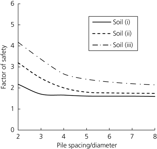
The variation of F_s with the ratio of pile-spacing to diameter (n = s/D; D = 0.3) is presented in Figure 11 for the case of soils (i)–(iii). As the soil-arching effect is more significant when the piles are placed closer, the resistance they offer will be greater. Therefore, higher F_s is found to occur at smaller pile-spacing. Further, it can be observed that, beyond the pile-spacing of 4–5D, the change in F_s is negligible, because of lower pile-contribution.

In this work, a new algorithm is proposed to compute the factor of safety of pile-stabilised slopes. The proposed algorithm involves an iterative procedure which models the progressive transfer of additional resistance offered by piles. The pile-stabilised slope is divided into three zones (pre-arching, arching and post-arching zone) and a pressure-based method proposed by Neeraj and Thiyyakkandi (2020) is extended to obtain the force on each zone. Thereby, the effect of soil arching on the load-transfer mechanism of pile-stabilised slopes was intrinsically incorporated in the proposed algorithm. The comparison between F_s values computed using the proposed algorithm and those obtained using finite-element modelling showed that the algorithm can be used as a quick, simple and reliable technique to estimate the factor of safety of pile-stabilised slopes. The conventional method of computing F_s wherein the pile-contribution is considered as an additional term, was found to over-predict the values. Unlike the conventional methods, the proposed algorithm incorporates the modified slip surface while computing the F_s, which significantly affects the estimated value. Subsequently, the variation of F_s with the pile location along the slope was studied. It was found that, for frictional soil, the mid-slope was the ideal location of the pile, while, as the cohesion value increased, the maximum F_s occurred when the piles were placed above the middle of slope. The factor of safety was found to reduce with an increase in pile-spacing due to poor contribution from the pile. Apparently, a pile-spacing greater than four to five times the diameter of piles was found to be ineffective in stabilising the pile. However, the optimal pile location and spacing should only be determined by studying other field constraints and the cost involved. The experimental validation of the proposed method is also warranted before field use.

The first author gratefully acknowledges the financial support provided by the Ministry of Education (MoE), India, for completion of this work.

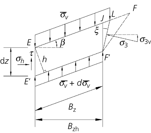
The enlarged view of the differential element EFF′E′ (Figure 2) is shown in Figure 12. The triangle LFF′ is in equilibrium state, and therefore, it can be ignored in the analysis of vertical equilibrium of the whole differential element (He et al., 2015a; Neeraj and Thiyyakkandi, 2020). The minor principal stress σ₃ acts on plane LF′, which can be resolved in vertical direction to obtain σ_3v as

Using the principles of origin of planes, it can be proved that:

$ξ=π4+φ2−θ1$⁠; $θ=12(φ−β+cos−1sinβsinφ)$⁠; and $θ1=12(φ+β+cos−1sinβsinφ)$

where θ is the angle between the slip plane and the slope surface; θ₁ is the angle between the slip plane and the horizontal; β is the slope angle; and φ is the angle of internal friction. Shear stress at face EE′ is given by:

Considering the vertical force equilibrium of the differential element dz,

Where B′ = (H − z) cos θ₁/sin θ and h = dzcos β.

Substituting Equation 26, Equation 2, Equation 25 and Equation 27 and rearranging,

C₁ and C₂ can be obtained from Equation 3.

Equation 22 is in the dy/dx + Py = Q form and can be integrated using the method of integration factor to obtain $σ¯v$⁠.

where, C is the constant of integration. Applying the boundary condition, $σ¯v=0$ at z = 0, in Equation 29 gives:

Substituting for C (Equation 30) in Equation 29 and re-arranging,

The resultant reaction on pre-arching zone, P_o, and the resultant lateral force transferred to the post-arching zone, P_i, can be obtained by integrating the force per unit length along the depth.

Here, σ_o and σ_i are the stresses along the outer and inner planes of the arching zone, respectively (Figure 1). The stress σ_i is given by Equation 2 and the stress σ_o is related to σ_i as (Neeraj and Thiyyakkandi, 2020):

Substituting Equations 2 and 33 in Equation 32 and integrating yields,

To obtain the points of application of these forces, the moment about the point where the piles intersect the slip surface is taken, that is,

Using Equations 2, 33–36, the point of application of forces from the slip surface can obtained as: