
Machine learning techniques establish the relationship between inputs and outputs in numerical simulations, circumventing the need for complex modelling and post-processing. This reduces the expertise and time required, facilitating wider adoption of numerical simulation methods. In this paper, taking the classic geotechnical engineering problem of slope safety factor calculation as an example, a comprehensive methodology for optimising numerical simulations using machine learning is presented. This includes: (a) the determination and quantification of input and output parameters for numerical simulations; (b) the design of the neural network, including the algorithm selection, the structure design, and the activation functions selection; (c) the design of training standards for neural networks; (d) the design of training and test sets using orthogonal and full factorial design methods; and (e) the model performance evaluation and the characteristics of prediction errors analysis. Furthermore, the probability of achieving the acceptable models on a training set and the extrapolation performance of the surrogate model are discussed in detail, which are beneficial for the design of the training sets and training sessions. The paper aims to standardise building and evaluating geotechnical numerical simulation surrogate models using machine learning, easing their application in engineering practice.
Notation
bias of the jth neuron in the hidden layer
bias of the output neuron
- c
cohesion of soil
errors in the network
- Fr
strength reduction factor
- Fs
slope safety factor
- f
activation function
- R2
coefficient of determination
- SSres
residual sum of squares
- SStot
total sum of squares of actual values
- t
horizontal coordinate of the slope crest
output of the jth neurons in the hidden layer
weights of the connections between the ith input and the jth neuron in the hidden layer
weights of the connections between the jth neuron in the hidden layer and the output neuron
- x
inputs of the BPNN
- y
outputs of the BPNN
actual value of the output
weight w and bias b adjustments during the backpropagation phase in the neural network
- η
learning rate
- φ
internal friction angle
Introduction
Numerical simulation has long been recognised as a powerful tool in geotechnical engineering for analysing the intricate behaviour of soil and rock, encompassing aspects such as slope stability, pile–soil interaction, and the deformation analysis of surrounding rock in tunnels. Typically, the utilisation of numerical simulation involves creating a geometric model, selecting an appropriate constitutive model, configuring contact properties, generating meshes, specifying boundary conditions, and post-processing the results. This operational procedure is labour-intensive and demands a profound level of expertise to guarantee the accuracy of each procedural step. Especially in the field of geotechnical engineering, a significant number of problems are non-linear in nature, which makes it necessary to consider the non-linear characteristics such as stress path dependence, anisotropy, time-dependence, and even fluid–structure coupling of soil and rock mass in numerical simulations. These factors collectively heighten the difficulty in obtaining accurate and reliable solutions in the numerical simulation of geotechnical engineering. Advanced expertise, substantial attempts, and extensive experience are indispensable in this process. Therefore, despite the acknowledged benefits of numerical simulation methods among experts and engineers, the widespread adoption of numerical simulations in practical engineering practices still faces significant obstacles.
Machine learning (ML) techniques hold the potential to overcome the limitations associated with the widespread adoption of numerical simulation. ML is a component of the artificial intelligence (AI) and endeavours to solve problems based on historical or given examples (Libbrecht and Noble, 2015). The basic application mode of ML is learning the hidden patterns or the mapping relationship between the input data and the output data and subsequently using the patterns or the mapping to classify or predict on new samples (Berry et al., 2020). Based on this application mode, ML has been successfully used across various fields, such as natural language processing, computer vision, speech recognition, recommendation systems, and autonomous vehicles (Asadi-Shekari et al., 2022; Ko et al., 2022; Lauriola et al., 2022; Pandey et al., 2022; Carrell et al., 2023; Hema and Garcia Marquez, 2023; William et al., 2023).
In the field of geotechnical engineering, the classical application of AI can be categorised based on the source of data into two types. The first type involves data derived from experiments or field observations, where ML is applied to unveil the relationships between experimental variables or observed parameters and outcomes, avoiding intricate theoretical analysis and calculations (Puri et al., 2018; Rauter and Tschuchnigg, 2021; Wu et al., 2021; Zhang et al., 2022c; Zhang et al., 2022b). The second type, emerging in recent years, focuses on data from numerical simulations, with scholars exploring the potential of AI techniques to construct relationships between inputs and outputs of numerical simulations in geotechnical engineering, offering significant insights (Gibson, n.d.; Zheng et al., 2021; Mitelman et al., 2023). However, they often do not concentrate on the process of developing practical surrogate models that can substitute for the numerical simulation, which is crucial for the wider adoption of numerical simulations in engineering practice. Moreover, these studies typically utilise a limited number of samples, ranging from a dozen to several dozens, which restricts a comprehensive evaluation of the AI-based model’s performance and offers limited guidance on achieving accurate and reliable surrogate models.
This paper attempts to provide a systematic and standard method, by which a reliable surrogate model of numerical simulation can be established based on the ML algorithm, to lower the application difficulties of numerical simulation and promote the application of numerical simulation technology in geotechnical engineering. To facilitate presentation, the calculation of slope safety factor was selected as an example in this paper. The structure of this paper is outlined as follows. Section 2 provides insights into the process of constructing a surrogate model based on the numerical simulation, including the determination and quantification of input and output parameters for numerical simulations, the initial configuration of the neural network, the training stopping criteria and training process, and the training and test sets design. Section 3 introduces methods for selecting the optimal model based on quantitative indicators (mean squared error (MSE) and R2) as well as approaches for analysing the error characteristics of the model. Section 4 offers an in-depth analysis of the likelihood of achieving acceptable models within a given training set as well as the performance degradation of surrogate models when applied to samples with input parameters beyond the scope of the training set.
Construction of the surrogate model
Numerical simulation method
A crucial step in building a database for ML is to define the input and output parameters. The input parameters of the database should be the key parameters for constructing the numerical model, which can uniquely define the numerical model and significantly influence the result. It usually includes parameters related to geometric shape and size, parameters reflecting material properties, parameters indicating contact relationships, parameters representing boundary conditions, parameters denoting load conditions, time parameters, and more. Excessive input parameters can increase the complexity of the AI model. Hence, it is crucial to simplify the number of parameters as much as possible and select a few representative key parameters as the input parameters for the database. The outputs should be extracted from the numerical simulation results according to a unified post-processing method to ensure consistency among different samples, guaranteeing the stability of the relationship between input and output data.
The slope safety factor computation, which is a classical problem in geotechnical engineering, was selected as the example of this paper. The software ABAQUS was selected as the tool to conduct the numerical simulation. ABAQUS supports Python-based modelling and post-processing programmes, and can automatically model and process results for multiple examples in batches, which is suitable for building a dataset containing a larger number of samples.
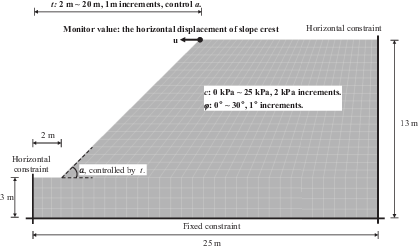
A typical two-dimensional numerical model for slope safety factor computation is shown in Figure 1. The inputs that may be involved in the slope safety factor computation include the physical and mechanical properties of the soil, the geometric shape of the slope, groundwater level, external load effects, environmental factors, and more. Considering all these factors as the input variables of the dataset will increase the complexity of the AI model, so simplification is necessary. The density of soil was kept constant, with a unit weight of 20 kN/m³. The Mohr–Coulomb model was adopted to represent the physical and mechanical properties of the soil; therefore, the cohesion c and internal friction angle ϕ were selected as the input variables to define the soil properties. The geometric shape of the slope was simplified by keeping the slope height and base width constant and using the horizontal coordinate of the slope crest t as the controlling parameter, which could effectively capture the influence of the slope angle a and facilitate the creation of modelling scripts by Python. Groundwater, external loads, and environmental effects are not considered in this model. In addition, the boundary conditions were consistent in all cases, with fixed vertical and horizontal freedom of the base and the horizontal degree of the two sides. Therefore, the database to be established had three inputs: the soil cohesion c, the internal friction angle ϕ, and the horizontal coordinate of the slope crest t. Other parameters, including describing the boundary condition and the gravity load, have been optimised out.
The other important issue is to quantitatively describe the results of the numerical simulation, which refers to the slope safety factor, denoted as Fs. In this paper, the Fs was determined utilising the strength reduction method, and the calculation process is described as follows:
- ▪
Step 1: Define a field variable, also referred to the strength reduction factor (Fr).
- ▪
Step 2: Specify the soil strength parameters (c, φ) that vary inversely with the field variable (Fr) defined in Step 1.
- ▪
Step 3: Establish the stress-equilibrium model by applying gravity with the initial Fr. Typically, the initial Fr value is set low to ensure a higher soil strength.
- ▪
Step 4: Gradually increase the Fr until the calculation fails to converge. Subsequently, the values of Fr obtained throughout the calculation process are analysed. Based on the instability criterion of the slope, the corresponding value of Fr at which the slope becomes unstable is used as the slope safety factor Fs.
There are generally two approaches to determining slope instability in Step 4 mentioned above. One approach is based on the trend or magnitude of the displacement of the slope crest, while the other approach is based on the distribution of the plastic zone on the slope model. Determining slope instability based on the distribution of the plastic zone makes it difficult to develop judgement programmes by Python and is more suitable for manual analysis. In this study, we have chosen the first approach to determine slope instability, which facilitates the development of a Python-based programme that could automatically extracting results. Initial efforts were made to use the inflexion point of the Fr–u curve as an indicator of slope instability, with the corresponding Fr at this inflexion point being considered as Fs. However, in some cases, there was no inflexion point in the Fr–u curve, and in other cases, algorithms such as finding the maximum derivative or using segmented fitting to determine intersection points could not accurately capture the correct inflexion point due to fluctuations in the curve. This made it extremely challenging to develop a unified automated programme for calculating Fs covering all cases. After multiple attempts, this study ultimately selected the Fr corresponding to the slope crest displacement of 10 mm as Fs. This choice was close to the inflexion point observed in most cases. For the cases where the calculation did not converge with the slope crest displacement of less than 10 mm, the Fr corresponding to the point at which the calculation ceased was used as Fs.
To verify the accuracy of the aforementioned method, a classical case presented by Dawson et al. (1999) was employed. In Dawson’s case study, the slope has a height of 10 m with 45° angle. The soil has a unit weight of 20 kN/m³, cohesive strength (c) of 12.38 kPa, and friction angle (ϕ) of 20°. Applying the limit equilibrium method, the calculated stability factor for this slope is 1, indicating a stable condition. Utilising the numerical simulation method and the algorithm for obtaining the slope safety factor described in this paper, the result of the Dawson case is 0.96, which is very close to the theoretical value of 1. This outcome serves as strong evidence to confirm the accuracy of the proposed simulation method and the approach for extracting the slope safety factor.
ML model configuration
ML techniques are defined as the discipline that enables computers to learn without explicit programming (Mahesh, 2020). Most scholars categorise ML techniques into three types: supervised learning, unsupervised learning, and reinforcement learning. Supervised learning, a fundamental category of ML, trains a model on a labelled dataset to make predictions and is mainly used for regression and classification problems (Sah, 2020). In contrast, unsupervised learning explores patterns and structures within unlabeled datasets and is mainly used for clustering and feature reduction (Udousoro, 2020). Reinforcement learning enables an algorithm to learn through interactions with an environment, receiving feedback in the form of rewards or penalties for specific actions. The most representative application of reinforcement learning is the video game (AlMahamid and Grolinger, 2021).
Using ML algorithms to build the surrogate model, which could reflect the relationship between the inputs and outputs of a numerical simulation, is a typical regression problem. Therefore, the supervised learning algorithms are suitable. In the supervised learning, algorithms capable of analysing regression problems include artificial neural networks (ANNs) (Li et al., 2020; Sedej et al., 2022), support vector machines (SVMs) (Zheng et al., 2021; Ben Seghier et al., 2023), and random forest (RF) (Rohmer et al., 2018; N et al., 2021). ANN is designed to mimic the information processing of the human brain. It consists of interconnected layers, including an input layer, one or more hidden layers, and an output layer. Neurons within each layer communicate with neurons in the subsequent layer through weighted connections (wij) and biases (bj) (Berry et al., 2020). SVM was proposed by Vapnik in the late 1960s (Rodriguez-Galiano et al., 2015). It is a supervised method to perform dichotomy classification of multi-dimensional feature vectors and utilises margin calculations to establish clear boundaries between classes. It draws margins, known as hyperplanes, to separate the classes effectively. The objective is to maximise the distance between the margins and the classes, ensuring a significant gap that minimises classification errors (Udousoro, 2020). The RF model, introduced by Breiman (2001), is a non-parametric ensemble classifier that extends the capabilities of the classification and regression tree algorithm. The RF combines multiple trees, each generated using bootstrap samples, resulting in improved performance and robustness (Mohammed and Ismail, 2021).
ANN is the most common algorithm in non-linear classification and regression problems (Rodriguez-Galiano et al., 2015). Although the performance of ANN may be slightly lower than other algorithms in some studies (Nitze et al., 2012; Rodriguez-Galiano et al., 2015; Mohammed and Ismail, 2021), it is relatively stable and not significantly lower than other algorithms in various types of complex problems. In addition, the adaptability of ANN on the training set containing noisy data is also better than other algorithms (Kurani et al., 2023), which means that the performance of the ANN algorithm may be more stable and reliable for complex non-linear problems. Therefore, in many comparative studies of ML methods, the ANN method is mostly used as a benchmark for comparison. Based on these considerations, the research in this paper selects the ANN method.
The backpropagation neural network (BPNN), a classical type of the ANN, employs the backpropagation of prediction errors across its multiple layers. BPNN leverages the chain rule from calculus to accurately determine the influence of each weight and bias on the cumulative error. Subsequently, adjustments to weights and biases are made in a direction opposite to the error gradient. This initiates a repetitive cycle involving a new prediction, a new error calculation, and a subsequent new weight and bias adjustment. The process continues until the prediction accuracy of the network reaches an acceptable level. Once this level is achieved, the BPNN is deemed to have effectively learned the relationship between inputs and outputs in the training dataset.
In the example of this paper, there were three inputs (t, c, ϕ) and one outputs (Fs). A BPNN with three inputs, one hidden layer consisting of 15 neurons, and one output was utilised. The rectified linear unit (ReLU) was selected as the activation function of the hidden layer. This activation function is a commonly used choice for regression problems, as it maps negative inputs to zero and effectively addresses the vanishing gradient problem (Pan et al., 2020). In addition, the output value of the ReLU function can be any positive number, making it suitable for regression problem compared with the sigmoid and hyperbolic tangent functions. The schematic diagram of this neural network is depicted in Figure 2. The x (×1, × 2, × 3) represents the input, the y denotes the output, the is the actual value of the output, the signifies the weights of the connections between the ith input and the jth neuron in the hidden layer, the refers to the bias of the jth neuron in the hidden layer, the signifies the weights of the connections between the the jth neuron in the hidden layer and the output neuron, and the refers to the bias of the output neuron.
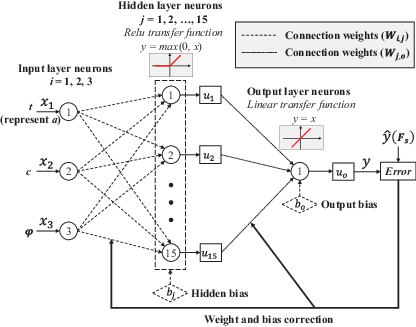
During the training of a BPNN, various mathematical formulas were employed, as detailed below. Equations 1–3 are employed in the forward propagation stage of the neural network. Equation 1 accounts for the calculation of output for neurons in the hidden layer, with f symbolising the activation function; Equation 2 represents the calculation of output for neurons in the output layer; Equation 3 denotes the calculation of errors in the network. Equations 4 and 5, respectively, represent the computations of weight w and bias b adjustments during the backpropagation phase in the neural network, with η symbolising the learning rate.
Training process configuration
The initial weights and biases significantly influence the final performance of a neural network. Inappropriate initial values could hinder the model from accurately capturing the relationship between the inputs and the outputs. Furthermore, this might even result in the failure of neural network training, signifying that the neural network could not fulfil the predefined training standards. Given the complex and varied relationships between inputs and outputs in different problems, no universally accepted methods currently exist to determine initial weights and biases. In practice, it is common to randomly assign initial weights and biases multiple times and decide on the final model based on its performance on the training and test sets.
In this study, the neural network designed in Section 2.2 was initialised with random weights and biases 1000 times for a specific training set. For each of these initialisations, the network underwent an iterative error correction process to reduce the MSE to below 0.01, resulting in 1000 distinct network models based on the given training set. Subsequently, the MSEs of 1000 networks on the test set were calculated, and the network with the lowest MSE on the test set was selected as the final model for the training set.
The MSE is a widely used indicator in ML to quantify the difference between predicted and actual values. It calculates the average of the squares of the errors between the predicted values and their corresponding actual values. The MSE provides a sensitive and comprehensive assessment of neural network performance by significantly amplifying larger deviations through the squaring operation, compared with other overall error evaluation indicators such as the root mean squared error (RMSE) and the mean absolute error (MAE) (Esparza-Gómez et al., 2023). Therefore, the MSE was selected as the main overall evaluation indicator. The calculation process for the MSE is presented in Equation 6. The is the actual value of the ith sample, and the is the prediction value of the ith sample.
Training and test sets design
Appropriate training set can reflect the relationship between inputs and outputs with fewer examples, reducing the workload of building the large training set and mitigating the risk of overfitting. Common methodologies for designing training samples include orthogonal and full factorial designs.
The orthogonal design, also known as the orthogonal array method or Taguchi method, is a systematic approach utilised in the design and analysis of sample selection across various fields. In the field of ML, the orthogonal experimental method has been commonly used to optimise the structure of the neural network (Pei et al., 2019; Rankovic et al., 2021) and reduce the required training sample size (Li et al., 2014; Liu et al., 2022). It features equilibrium dispersion and neat comparability, which enable it to offer a comprehensive understanding of the relationship between inputs and their outputs while minimising the required sample size. The full factorial design, also known as the fully crossed design, represents another method employed in constructing training sets (Kreutz et al., 2020; Kosarac et al., 2022). Compared with orthogonal design, full factorial design provides a more thorough and accurate analysis of the relationship between inputs and their outputs by considering all possible combinations of factor levels, despite leading to a greater number of samples compared with the orthogonal design under the same number of levels. Both orthogonal design and full factorial design aim to capture the impact of inputs on outputs, and could be utilised to design the training set.
In applying the orthogonal or full factorial design to determine the training set with the minimum size, the common strategy is gradually increasing the number of each input levels from fewer to more. This process is continued until the model’s performance ceases to show significant improvement and the associated performance indicators reach acceptable thresholds. This strategy effectively identifies the optimal training set that provides a reliable representation of the input–output relationship without unnecessarily enlarging the dataset.
To clearly explain the process of developing a reliable surrogate model with an optimal training set, this study methodically designed training sets based on the orthogonal and full factorial design across several levels: 3, 5, 7, 9, 11, 13, and 15. Each input variable has the same number of levels in a training set. For example, in a training set with three levels, the input variables t, c, and ϕ each have three distinct values. The performance of models based on different training sets would be compared. Details for the values assigned to input variables of each training set are provided in Figure 3. There are various methods for designing Taguchi array, and the resulting sample sizes vary depending on the specific approach. The Taguchi array used in this study is based on the method described in literatures (Leung and Wang, 2001; Chixin, 2019). The number of samples in each training set is shown in Table 1. It should be pointed out that in practice, the level of the training set is usually gradually added based on the performance of the network on the training set, and there is no need to design training sets with multiple levels in advance.
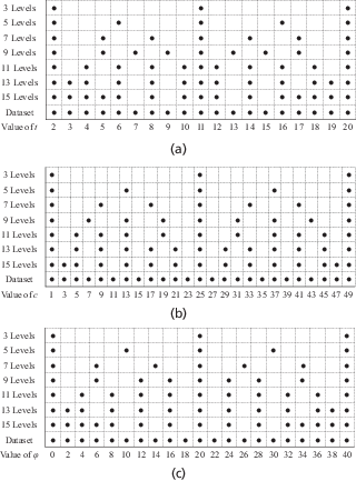
Values of each input in the different training set designs and the overall dataset. (a) The values of t. (b) The values of c. (c) The values of ϕ
Values of each input in the different training set designs and the overall dataset. (a) The values of t. (b) The values of c. (c) The values of ϕ
The number of samples in each training set
| Levels | Orthogonal design | Full factorial design |
|---|---|---|
| 3 | 9 | 27 |
| 5 | 25 | 125 |
| 7 | 49 | 343 |
| 9 | 81 | 729 |
| 11 | 121 | 1331 |
| 13 | 169 | 2197 |
| 15 | 225 | 3375 |
A database encompassing all training sets was established, with the values of each input parameter displayed in Figure 3. This database contains a total of 9975 samples. The dataset includes a range for t from 2 to 20 m, incremented by 1 m; for c from 1 to 49 kPa, incremented by 2 kPa; and for ϕ from 0° to 40°, also incremented by 2°. For any given training set, its test set comprises all other cases in the database not included in that training set. The ratios of the test set to the training set are maintained above 1:4 on each design of training set, a ratio generally considered as the minimum acceptable for the test set, to ensure a thorough evaluation.
Determination of the surrogate model
Optimal model selection
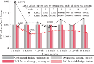
Utilising the methodology presented in Section 2.3, the optimal models for each training set were identified. Figure 4 illustrates the MSE values of these optimal models on both their respective training and test sets. Analysis of Figure 4 yields the following insights. First, the MSE values for each model on its training set were slightly below 0.01, with minimal variance among the models. This observation aligns with the predetermined training termination criteria, indicating that each model was adequately trained to meet these criteria and demonstrated a good fit for the training set. Second, the performance of the models on their test sets exhibited significant differences. For training sets designed using orthogonal arrays, the MSE values on the test sets decreased from 0.1973 to 0.0088 as the training sets expanded from three levels to nine levels, marking the lowest value achieved in this study. With the training sets increasing from 9 to 15 levels, the MSE on the corresponding test sets showed fluctuating trends, consistently exceeding the MSE of 0.0088 observed on the model trained by the nine-level training set. For training sets constructed by way of full factorial design, the lowest MSE (0.0063) on the test sets was observed on the five-level training set. Beyond five levels, the MSE on the test sets initially increased and then decreased, with the magnitude of change being relatively small. The observed deterioration trend of MSE beyond a certain number of levels, evident in both models derived from orthogonal and full factorial designs, suggests the possibility of overfitting. However, other factors, such as the complexity of the model, the optimisation algorithm used, or imbalances in the data distribution, may also contribute to this phenomenon. Third, under the same number of levels, models trained on datasets generated from full factorial designs demonstrated better performance (a lower MSE) than those from orthogonal designs. As the number of levels increased, the discrepancy in MSE between models based on orthogonal design and full factorial design tends to decrease but was still large, indicating that increasing the number of levels can improve the training effect of the training set derived by orthogonal design, but the improvement was limited. Furthermore, to achieve similar MSE values, the number of cases in the training samples from full factorial designs was substantially less than those from orthogonal designs. For instance, the nine-level training set based on the orthogonal design included 81 cases, resulting in an MSE of 0.0088 on the test set, whereas the three-level full factorial design training set comprised only 27 cases, with an MSE of 0.0091 – a mere difference of 0.0003. This indicates that, for the slope stability problems addressed in this study, constructing training sets by way of full factorial designs is far superior to using orthogonal designs.
The coefficient of determination R2 means, also known as R-squared, is a statistical measure used to evaluate the goodness-of-fit of a regression model. In the neural networks, the R2 is employed alongside the MSE to provide a comprehensive assessment of the model’s predictive accuracy. Distinguished from the MSE, RMSE, and MAE, which measure the overall difference between the real and predicted values, the R2 evaluates the fit of the neural network model to the variability of the data. R2 = 1 indicates a perfect fit, meaning that the neural network can explain all the variability in the target variable. Conversely, R2 = 0 means that the neural network cannot explain any of the variability. The detailed computing process of R2 is denoted by Equations 7–10. The SStot is the total sum of squares of actual values; the SSres is the residual sum of squares, which measures the discrepancy between the predicted values and the actual values. The R2 of each model on its training set and response test set was calculated and presented in Figure 5.
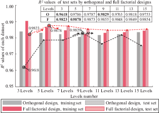
Analysis of the R2 value for each model on their respective training and test set yielded the following conclusions. (1) The R2 values for each model on their training sets were above 0.98, indicating that the models were sufficiently trained and capable of accurately reflecting the data trends in the training sets. First, the R2 on the test set exhibited a variation pattern similar to that of the MSE. For models based on orthogonal design, R2 on the test set increased with the number of levels (indicating improved performance) until it peaked at nine levels (0.9829), after which it fluctuated, with all subsequent values being lower than the R2 at nine levels. For the full factorial designs, the models corresponding to five levels achieved the highest R2 (0.9878) on its test set, and beyond that, as the number of levels increased, R2 showed a trend of initially decreasing slowly and then increasing slowly. This still suggests that, whether for orthogonal or full factorial designs, models’ performance decline after reaching a certain number of levels in the training set. In addition, similar to the characteristics of MSE, training sets from full factorial designs outperformed those from orthogonal designs at the same number of levels, especially when the number of levels was low, where the performance gap was more pronounced.
Combining the analysis of MSE and R2 across various levels, the model trained on the training samples derived from a full factorial design with five levels was found to have the smallest MSE and the highest R2 on the test set, making it the optimal model obtained in this study. The detailed parameters of this model are presented in Table 2.
The connection weights and biases of the optimal model in this study
| Hidden neuron | Weight | Bias | ||||
|---|---|---|---|---|---|---|
| Input1-t | Input2-c | Input3-ϕ | Output | Input | Output | |
| 1 | −0.572 | −0.894 | 0.223 | −0.232 | 0.714 | 0.196 |
| 2 | −0.963 | −0.076 | 0.431 | −0.275 | 0.560 | — |
| 3 | −0.906 | −0.078 | −0.741 | 0.392 | 0.355 | — |
| 4 | −0.206 | −0.134 | −0.173 | 0.648 | −0.108 | — |
| 5 | 0.089 | 0.329 | −0.315 | 0.560 | −0.733 | — |
| 6 | 0.450 | 1.048 | −0.625 | −0.008 | 0.014 | — |
| 7 | −0.405 | 0.071 | −0.263 | −0.864 | 0.186 | — |
| 8 | −0.076 | 0.826 | 0.240 | −0.018 | −0.111 | — |
| 9 | −0.173 | 0.125 | 0.117 | −0.007 | −0.648 | — |
| 10 | −0.749 | −0.391 | −0.192 | 0.065 | 0.965 | — |
| 11 | 0.932 | 0.427 | 0.188 | 0.325 | −0.759 | — |
| 12 | 0.203 | −0.473 | 0.193 | 0.535 | 1.139 | — |
| 13 | 0.364 | −0.609 | −0.362 | −0.037 | −0.532 | — |
| 14 | 0.129 | −0.631 | −0.456 | −0.897 | 0.987 | — |
| 15 | 0.254 | 0.040 | 0.107 | −0.689 | −0.755 | — |
Error distribution characteristics analysis
MSE and R2 serve as quantitative overall evaluation indicators that reflect the overall performance of a model, and they are unable to further analyse the detailed error characteristics of a model, such as which conditions result in higher prediction accuracy or which factors affect the model’s accuracy. However, these error distribution characteristics are very important for evaluating the availability or determining the applicable conditions of the surrogate model. Visual charts are frequently employed to conduct a detailed analysis of the distribution characteristics of prediction errors generated by a model. They could offer intuitive insights into the model’s accuracy, revealing patterns and discrepancies not immediately evident through numerical indicators alone.
Figure 6 illustrates the error distribution of the optimal model (five levels, full factorial design) within the test dataset. The horizontal axis represents the magnitude of the error, defined as the predicted value minus the actual value, while the vertical axis shows the percentage of samples falling into specific error ranges relative to the total number of samples in the test set. Figure 6 reveals the following key characteristics of the optimal model’s error distribution. First, the majority of errors are concentrated in the ±0.1 range, with samples within this interval constituting 81.81% of the total, indicating that the model generally exhibits high predictive accuracy. Second, the distribution of errors reveals a bias towards underestimation of the slope safety factor, with 60.1% of the errors being negative (predicted values are less than actual values) and 39.9% being positive (predicted values exceed actual values), exhibiting a conservative bias in the model’s prediction. Third, two significant outliers (identified as outlier1 and outlier2) are observed, exhibiting errors of 1.09 and 1.79, respectively, which are considerably larger than those seen in other samples. These outliers correspond to samples with inputs: t = 8 m, c = 27 kPa, ϕ = 22°; and t = 8 m, c = 43 kPa, ϕ = 28°. This observation underscores the necessity of enriching the training set with additional samples near these parameter values to enhance the model’s predictive capability in similar scenarios.
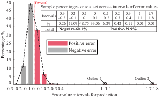
Figure 7 presents a scatter plot of actual against predicted values for the surrogate model on the test set, where each point represents an individual sample. Analysis of Figure 7 yields the following insights into the characteristics of the model’s prediction error. First, the majority of data points are closely aligned with the reference line (y = x, where the actual value equals the predicted value), indicating a strong agreement between the model’s predictions and the actual values. This alignment suggests that the model is capable of accurately reflecting the trends within the test dataset. This observation is further supported by the model’s R2 value of 0.9878, which signifies a high degree of fit to the test data. Second, there is a noticeable trend of sample points increasingly clustering near the reference line (y = x) as the actual values rise, indicating that the model’s predictive accuracy is influenced by the magnitude of the actual values. This suggests that the model tends to achieve more accurate predictions for higher actual values.
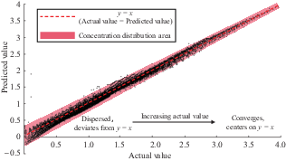
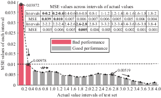
Figure 7 suggests a potential correlation between the magnitude of prediction errors and actual values, potentially indicating the model’s applicability range. To explore this relationship further, this study categorised the test set into several groups based on the magnitude of actual values, using intervals of 0.2, and calculated the MSE for each. The results, depicted in Figure 8, lead to the following conclusions. First, the MSE distribution divides at an actual value threshold of 0.4, delineating two distinct regions of error magnitudes. The MSE is significantly higher for actual values less than 0.4 as compared with actual values greater than 0.4. Within the range of actual values less than 0.4, the MSE for the interval between 0 and 0.2 is markedly higher than that for the interval between 0.2 and 0.4. Second, the trend in MSE across the intervals shows a sharp decline for actual values between 0 and 0.4, followed by a gentle fluctuation for values between 0.4 and 2.6, and then a significant decrease again. Overall, the model’s predictive accuracy is deemed reliable for actual values exceeding 0.4 and further enhanced with increasing actual values, achieving peak reliability beyond 2.6. However, it is important to note that the model exhibits reduced accuracy in predictions when the actual values are below 0.2, necessitating cautious judgement.
Further discussions on the surrogate model construction
Probability of obtaining acceptable models
Section 3.1 conducts a comparative analysis of model performance across various training sets. The analysis focuses on two indicators (MSE and R2), without discussing the probability of obtaining an acceptable model on a training set. In the study, neural networks were randomly assigned initial weights and biases 1000 times on the same training set. Following each initialisation of weights and biases, the network autonomously iterated until the MSE fell below 0.01, resulting in 1000 initial models. Although the 1000 models achieved acceptable performance on the training set, significant variability was observed in their performances on the corresponding test set. Among these 1000 models, the proportion that achieved acceptable performance on the test set is defined as the probability of obtaining an acceptable model on a training set (hereinafter referred to as probability) in this paper. It was observed that the probability varies across different training sets.
Figure 9 illustrates the probability distribution of performance indicators (R2 and MSE) for 1000 models on a test set, which are generated by initialising weights and biases 1000 times on the corresponding training set. Performance was categorised as follows: for MSE, excellent (<0.01), good (0.01 to 0.1), fair (0.1 to 0.5), and poor (>0.5); for R2, excellent (>0.9), good (0.8 to 0.9), fair (0 to 0.8), and poor (<0), with R2 values below 0 indicating an inability of the model to fit the test data trend.
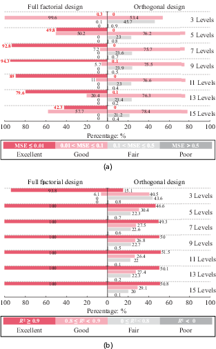
Distribution of test set MSE and R2 across 1000 training sessions for models on various training sets. (a) MES ditribution. (b) R2 ditribution
Distribution of test set MSE and R2 across 1000 training sessions for models on various training sets. (a) MES ditribution. (b) R2 ditribution
Analysis of MSE distribution in Figure 9 yields two key findings. (1) Models trained on datasets employing a full factorial design demonstrate a higher likelihood of achieving better performance. For instance, in achieving models classified as excellent, each training set designed by the full factorial design presents a certain probability. Conversely, for orthogonal design, only the 9-level and 13-level training datasets have a 0.1% (only 1 among 1000 models) chance of achieving it. (2) The likelihood of achieving models with better performance on the training set does not exhibit a strictly positive correlation with the number of input levels. For example, in the full factorial design, the probability of attaining models classified as excellent peaks at nine levels, reaching a maximum of 94.3%, and a marked decline in this probability appears with the increasing in the number of levels. This suggests that an increased sample size does not guarantee a higher likelihood of developing models with superior performance.
Similar patterns are observed in the R2 distribution, with full factorial designs outperforming orthogonal designs in producing models with better performance. Notably, the chance of achieving models with excellent R2 performance reaches 100% at five levels in full factorial designs and remains constant thereafter, whereas in orthogonal designs, the probability significantly increases from 15.1% at three levels to 49.3% at seven levels, then slightly rises to 51.5% between 7 and 11 levels, before slightly decreasing.
Theoretically, a neural network, when configured with a predefined basic setup, is capable of modelling data trends using training sets of any size and derived through various design methodologies. Nonetheless, the likelihood of successfully training such models is significantly affected by the characteristics of the training set, including its design methodology and size. This analysis confirms this viewpoint, highlighting the importance of carefully selecting the number of training sessions, defined as the number of times the initial weights and biases are randomly assigned. Insufficient training sessions may lead to failure to achieve the model with excellent performance on the given training set.
Extrapolation performance of the surrogate model
The extrapolation performance of neural networks refers to the model’s ability to predict data outside the range of the training set. In constructing the surrogate model presented in this paper, the input data for the test set were all within the range of the training set, and the performance of the model on the samples beyond the training set was not discussed. This scenario is likely to occur in practical applications of the surrogate model. To thoroughly explore characteristics of the model’s extrapolation performance, this study redesigned multiple training and corresponding test sets, conducting a detailed analysis of the model’s performance during single-parameter extrapolation and full extrapolation across all three parameters.
This section encompasses four analyses related to the study. Analysis 1 evaluates the model’s performance when all three input variables (t, c, ϕ) are outside the range of the training set data. Analysis 2 investigates the model’s performance when the slope crest horizontal coordinate t is beyond the training set’s range. Analysis 3 assesses the performance of the model when the cohesion c is not within the range of the training set. Finally, analysis 4 examines the model’s performance when the internal friction angle ϕ falls outside the training set’s scope. The specific inputs values of the various training sets, test sets, and extrapolation sets involved in the study are illustrated in Figure 10.
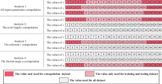
The values of input parameters in the study of neural network extrapolation performance
The values of input parameters in the study of neural network extrapolation performance
In the aforementioned four analyses, the models employed were selected based on achieving the minimum MSE on their respective test sets, following 1000 iterations of random initialisation of weights and biases and subsequent training until satisfying the predefined conditions, as described in Section 2.3. Then, about 20% of the samples from the training set are used for preliminary testing of the model. From the 1000 preliminary models generated, the model with the best performance is identified based on the MSE value. This model is considered the optimal model achievable with the given training set. Furthermore, to more clearly demonstrate the models’ extrapolation performance, the optimal model determined in Section 3, which was developed using a training set designed by five-levels full factorial design method, was served as the benchmark for performance when extrapolating without any input parameters. The MSE and R2 for each model, when extrapolating with one input parameter and with all three parameters outside the training set, are depicted in Figure 11. In addition, the MSE and R2 values for each model on the test set are also shown in Figure 11 to demonstrate their performance when no input parameter falls outside the training set.
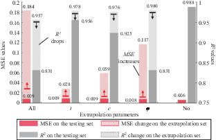
Analysis of Figure 11 leads to the following conclusions. All models exhibited good prediction performance on the test set, where all input parameters fall within the range of training data. The MSE for all models on the test set was below 0.01, and the R-squared values were all above 0.95. However, when evaluating the models on the extrapolation dataset (where input parameters extend beyond the range of training data), a significant performance degradation was observed across all models. This decline in prediction accuracy was particularly pronounced when all three input parameters were outside the training range, resulting in a significant increase in MSE from 0.009 to 0.184 and a decrease in R2 value from 0.957 to 0.831. Furthermore, the extent of performance deterioration varied for individual input parameters exceeding their respective training ranges. Notably, the model exhibited the most significant decline in performance when the internal friction angle (ϕ) was outside the training range. The parameter extrapolation significantly influences model prediction accuracy and modestly impacts the model’s data-fitting capability.
Figure 11 presents the influence of input parameter extrapolation on model prediction accuracy. To further analyse this issue, the error distributions of the models on the extrapolation sets when extrapolating with one and all three parameters outside the training set range were presented in Figure 12. The horizontal axis of Figure 12 categorises errors into intervals of 0.1, while the vertical axis represents the percentage of samples within each error interval relative to the total number of samples in the test set. Analysis of Figure 12 yields the following conclusions. (1) The error range of the model noticeably expands on extrapolation sets with extrapolated input parameters. With all three parameters extrapolated, the error range is −0.7 to 1.1 (not considering one outlier sample). With only t extrapolated, the error range is −0.6 to 0.6. With only c extrapolated, the error range is −1.4 to 0.6 (not considering one outlier sample). With only ϕ extrapolated, the error range is −1 to 1.2. On the contrary, when parameters are not extrapolated, the error range is −0.3 to 0.4 (not considering two outlier samples). This indicates an increased predictive error in the model on datasets outside the training set. The extent of this increase depends on which and how many parameters are extrapolated. (2) The model’s predictive accuracy is substantially influenced by input parameters extrapolation. When all parameters are extrapolated, only 15.43% of the samples lie within an error range of ±0.1, compared with 49.1% for just t extrapolation, 43.92% for just c extrapolation, 27.95% for just ϕ extrapolation, and 81.81% when parameters are not extrapolated. Overall, Figure 12 indicates a significant reduction in model accuracy on samples with extrapolated input parameters, in terms of increased error and the reduced proportion of accurate predictions. This effect depends on the number and specific parameters extrapolated, with more extrapolated parameters leading to a larger impact.
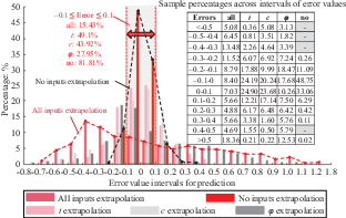
The distribution of prediction error on the test set under different input parameters extrapolation
The distribution of prediction error on the test set under different input parameters extrapolation
The analysis of the model’s performance on extrapolation sets suggests that the coverage range of input parameters in the training samples should be expanded as much as possible during training set design. Also, after constructing the numerical simulation surrogate model, its applicable parameter range should be clearly stated to prevent the degradation of predictive ability when input parameters are extrapolated.
Recent research in ML has demonstrated the effectiveness of incorporating prior information or uncertainty into data-driven models to enhance their generalisation ability (Raissi et al., 2019; Liu Yang et al., 2021; Meng et al., 2021; Zhang et al., 2022a; Zhang et al., 2024). These studies highlight the potential for integrating domain-specific knowledge into ML models to improve their performance and broaden their applicability. This approach holds significant promise for advancing the development of geotechnical numerical simulation surrogate models, particularly in terms of improving extrapolation performance and reducing model uncertainty.
Conclusion
This paper provides a detailed introduction to the use of ML to build numerical simulation surrogate models for geotechnical engineering and discusses some issues encountered during the process of the surrogate model construction. The surrogate model, which is based on the numerical simulation, allows the user to obtain results that are fairly close to those of numerical simulation with simple input parameters. It avoids the complex and specialised process of numerical simulation, significantly reducing the time and learning cost needed to apply numerical simulations, and encourages the further promotion of numerical simulation methods. Taking the classical geotechnical engineering problem of slope stability analysis as an example, the work conducted and conclusions drawn in this paper are as follows.
- ▪
This paper provides a detailed discussion on the construction of numerical simulation surrogate models for geotechnical engineering using ML methods, including constructing and determining the model. The construction process involves: (a) the determination and quantification of input and output parameters for numerical simulations; (b) the design of the neural network, including the algorithm selection, the structure design, and the activation functions selection; (c) the design of training standards for neural networks; and (d) the design of training and test sets using orthogonal and full factorial design methods. The determination of surrogate models primarily encompasses the model performance evaluation, selection of the optimal model, and analysis of model error characteristics.
- ▪
The probability of achieving acceptable model performance on the same training set was discussed. Theoretically, by increasing the number of random assignments for initial weights and biases, it is possible to achieve satisfactory models on any training sample given unchanged network settings and training standards. However, the probability of achieving acceptable models is greatly influenced by the design method and size of the training samples. In the case studies of this paper, this probability was extremely low for training samples designed using orthogonal design, but relatively higher for those based on full factorial design. In addition, the analysis in this paper indicates that the relationship between this probability and sample size is not strictly positive, meaning that the probability of obtaining acceptable models does not continuously increase with larger sample sizes. These findings offer insights into the design of training samples and the number of neural network training sessions (the number of random assignments for initial weights and biases).
- ▪
The performance of the surrogate models on samples outside the training set range was analysed. Analysis indicates a significant decrease in predictive capability when input parameters fall outside the training set range, especially in terms of prediction accuracy (error magnitude and the proportion of small errors). The extent of performance degradation is related to the number of extrapolated parameters and which specific parameter is extrapolated. The performance degradation is more pronounced when there are more extrapolated parameters.
Funding
This research was supported by the Support for Scientific Research Start-up for Talents Recruitment of Nanjing Vocational University of Industry Technology (NO. YK22-06-01) and Nanjing Construction Industry Science and Technology Planning Project (NO. Ks2318; Ks2261).
Conflict of interest
The authors have no competing interests to declare that are relevant to the content of this article.
Authors’ contributions
Kunpeng Gao led the conceptualisation and methodology design, and drafted the manuscript. Zhiyuan Cheng and Yihua Song contributed to data analysis and significantly revised the manuscript after the first review. Shuhui Yin and Yihao Chen were responsible for data organisation and the creation of figures. All authors reviewed and approved the final manuscript.


