There is mounting evidence in favour of replacing the e against diagram, conventionally used to represent soil compressibility in an oedometer, with a log(v) against diagram, which significantly improves the linearity of virgin loading and unloading paths. This paper presents a simple, new formulation of the ‘intrinsic’ compression and ‘sedimentation’ compression lines for a range of insensitive, sedimentary marine clays presented in Burland’s 1990 Rankine Lecture by using a log(v) against interpretation of the data.
Notation
- Cc
virgin compression index in the traditional plane
natural compression index for virgin compression on the plane
intrinsic compression index
- ,
intrinsic compression indices on the plane for the reconstituted (r) and natural (n) samples, respectively
- e
void ratio
void ratio corresponding to
void ratio corresponding to
- eL
void ratio at liquid limit
- Iv
void index
- LL, wL
liquid limit
- log(S)
spacing between the intrinsic compression and sedimentation compression lines in the model
- mv
coefficient of volume compressibility; m vr for reconstituted and m vn for natural samples
- v
specific volume; v r for reconstituted and v n for natural samples
- v0
reference specific volume on the virgin compression line
- vL
specific volume at liquid limit
- ,
intrinsic specific volumes of the reconstituted and natural samples, respectively, corresponding to
- w
water content
effective vertical stress
reference effective vertical stress on the virgin compression line
Introduction
When samples of argillaceous soils are recovered, often in a disturbed state, it is a relatively simple matter to dry the soil, reconstitute samples of it (typically with water contents at, or up to 1·5 times, their liquid limit) and determine from them compressibility parameters in virgin compression in an oedometer. Such soils are often found, normally consolidated, in a marine environment having undergone only sedimentary compression. It is of considerable interest, and practical importance, to determine whether or not there is a consistent relationship between the void ratio, or specific volume, of the reconstituted soil, undergoing vertical effective stress increments in virgin confined compression, and the corresponding relationship for the same soil in its natural in situ state.
Skempton (1970) published sedimentation compression curves covering a wide variety of such deposits and effective consolidation pressures ranging over five orders of magnitude. Subsequently, Burland (1990) presented his concept of an intrinsic compression line (ICL), for reconstituted samples, and a sedimentation compression line (SCL), for a wide range of natural sedimentary clays, as a means of normalising and comparing the two families of results. The ICL and SCL, although not straight, were found to be closely parallel, enabling the more readily determined ICL parameters to be used to predict those for the same soil in its natural state.
Embedded in Burland’s analysis is an empirically extrapolated curve passing through two points on the e against plot for soil in confined compression, within the vertical effective stress range of 100 kPa ≤ ≤ 1000 kPa, as a means of overcoming the fact that e against curves for such soils, over a wider range of effective vertical stress, are usually non-linear.
The present paper presents a reformulation of Burland’s proposal in which the compression data are plotted in a log(v) against diagram, with v = (1 + e), in the form
where is a reference point on the virgin compression line and is the relevant natural compression index for virgin compression.
It was established by Butterfield (1979, 2011) and subsequently confirmed, also recently by Suddeepong et al. (2015), that such a interpretation of the data offers a much improved linearity (closely linear plots) for many soils (in particular clay and silty–clay soils) over a wide range of values; a gradient that generates natural strains directly and is therefore applicable to large strain deformation; compression equations that are independent of the base of the logarithms used for plotting; and a satisfactory interpretation of the earlier-mentioned difference in soil stiffness.
When the Burland (1990) and Skempton (1970) data are interpreted in this way, both the equivalent ICL and SCL are found to be closely parallel straight lines. In fact, they become merely normalised log(v) against plots, and their presentation is thereby both clarified and simplified.
Intrinsic parameters for a class of reconstituted clays
Review of Burland’s analysis
In his 1990 Rankine Lecture, Burland presented the ICL as a means of unifying virgin compression data obtained on a class of reconstituted clays. These were normally consolidated insensitive marine clays, reconstituted by thorough mixing at a water content at least as high as their liquid limit, with Atterberg limits (w L%, PI%) lying slightly above the A line in a Casagrande plasticity chart.
Burland introduced the following parameters to define the ICL
two intrinsic void ratios, and , defined as the void ratios of each reconstituted soil corresponding to and 1000 kPa, respectively, together with their intrinsic compression indices
, being the value of C c for a line joining the above points in an e against diagram.
These three new parameters were then used to define a further one, the void index (I v), as
Burland’s ICL results from plotting I v against , with in kilopascals. Figure 1(a) shows his oedometer test data for six such clays, spanning a wide range of liquid limit values, when reconstituted at a water content w with (w L < w < 1·5w L). Figure 1(b) is the ICL that they generate. It is interesting to note that had the plots been linear, then, since , one would have , and the ICL equation would become simply
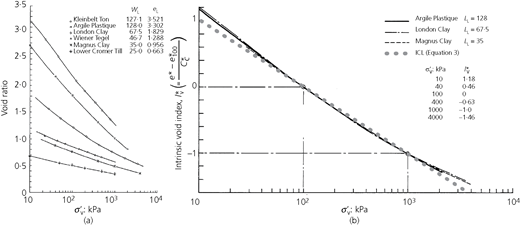
(a) One-dimensional compression curves for various reconstituted clays, from Burland (1990). (b) Normalised intrinsic compression curves giving the ICL of Equation 3 (dotted gray line). L L, liquid limit
(a) One-dimensional compression curves for various reconstituted clays, from Burland (1990). (b) Normalised intrinsic compression curves giving the ICL of Equation 3 (dotted gray line). L L, liquid limit
This straight line has been added to Figure 1(b), providing (dotted gray line), as expected, an acceptable fit to the data between and and departing from it as the linearity of the e against curve breaks down. The actual ICL is curved, and Burland (1990) provides a fitted cubic equation for it in terms of as
A log(v) against interpretation
If the data on the virgin compression of the reconstituted clays are interpreted in terms of the log(v) against model, the result is very closely a straight line with gradient , replacing ; the subscript r attributing the parameter to the reconstituted soil. An equivalent linear version of Figure 1(b) can then be generated by introducing one further parameter . By analogy with , becomes the ‘intrinsic specific volume’ of the reconstituted clay corresponding to .
If is redefined as atmospheric pressure = 100·33 kPa, this will have a negligible numerical effect on established results while removing the restriction on the units of to kilopascals. The form of Equation 1 also means that the use of base 10 logarithms in calculations and plotting is no longer mandatory.
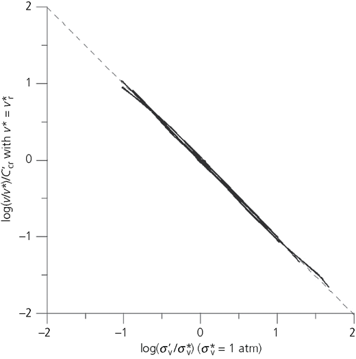
Figure 2 shows the Figure 1(a) data plotted on axes, where it becomes, very closely, a set of straight lines converging at around (5·6, 0), each with a soil-specific gradient . The data can be normalised by plotting against as shown in Figure 3. This is a straight-line, alternative form of the ICL (say, ICL*, the ICL in the model) with gradient = −1, passing through the coordinate origin with the equation
in which are specific (intrinsic) to each clay and v represents v r, the specific volume of a reconstituted sample. Equation 5, analogous to Equation 3, is seen to be simply a normalised version of Equation 1.
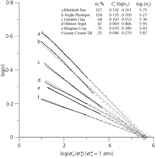
Lines generated from the reconstituted clays data set of Figure 1(a) plotted on the plane (thick continuous lines: original data set; thin continuous lines: Burland’s fitting; thin dashed lines: new fitting)
Lines generated from the reconstituted clays data set of Figure 1(a) plotted on the plane (thick continuous lines: original data set; thin continuous lines: Burland’s fitting; thin dashed lines: new fitting)
Oedometer tests on the reconstituted soils provided values of , and these correlate reasonably with their specific volume at liquid limit (v L) to provide the relationships
These expressions are analogous to those quoted by Burland (his Equations 4 and 5) for estimating his parameters from e L using the same data.
Intrinsic parameters for a class of naturally sedimented clays
Burland’s analysis
The next stage of Burland’s (1990) development was to use the earlier-presented empirical correlations to estimate the values of and for a collection of natural marine clays for which e L was known. For this purpose, he used an augmented set of the large collection of data on normally consolidated argillaceous sediments published by Skempton (1970). Since the in situ void ratio and the associated effective overburden pressure were also known for each data point, Burland was able to estimate for each point from e L and hence calculate another void index for the natural clays and plot it against for each of them.
The result of the process is shown by the points in Figure 4.
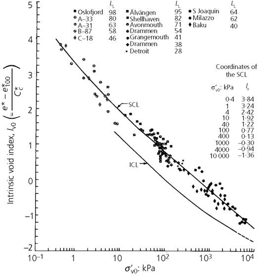
Relationship between I v0 and for many of the normally consolidated clays designated in Skempton (1970) and SCL as in Burland (1990)
Relationship between I v0 and for many of the normally consolidated clays designated in Skempton (1970) and SCL as in Burland (1990)
He fitted a curve through them, which, by analogy with his ICL (also shown in the figure), he called the SCL. This can be plotted from the interpolation table shown in the figure. His ICL and SCL are approximately parallel, from which he concluded that ‘at a given value of void index I v0 the effective overburden pressure carried by the natural clay is approximately five times that carried by the equivalent reconstituted clay’ (Burland, 1990: p. 340).
A log(v) against interpretation of Figure 4
Figure 5 shows the complete, augmented, natural-clay data set, digitised from Skempton’s (1970) database and replotted for each individual soil (thick lines) in terms of log(v) against , omitting the individual data points. Because the natural-clay soil samples covered a range of depths at each site, an approximate (light) line can be fitted to each set to provide a site-specific value of, say, natural compression index and (the specific volume under ). This diagram can be normalised, in the same way as the reconstituted samples, by plotting against as in Figure 6 (v here designating the value of v n for a natural soil). The result is again very closely a straight line, which can be fitted by Equation 5 when are replaced by – that is
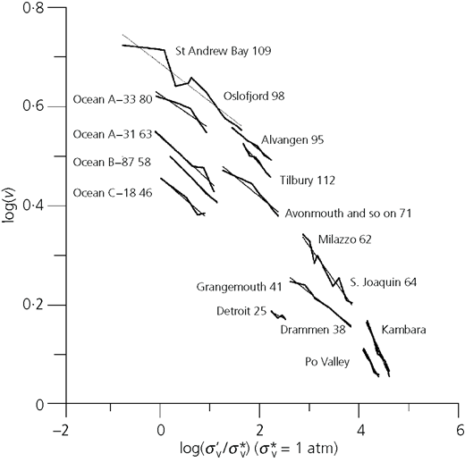
Complete natural-clay data set (thick lines) plotted together with fitted log(v) against lines
Complete natural-clay data set (thick lines) plotted together with fitted log(v) against lines
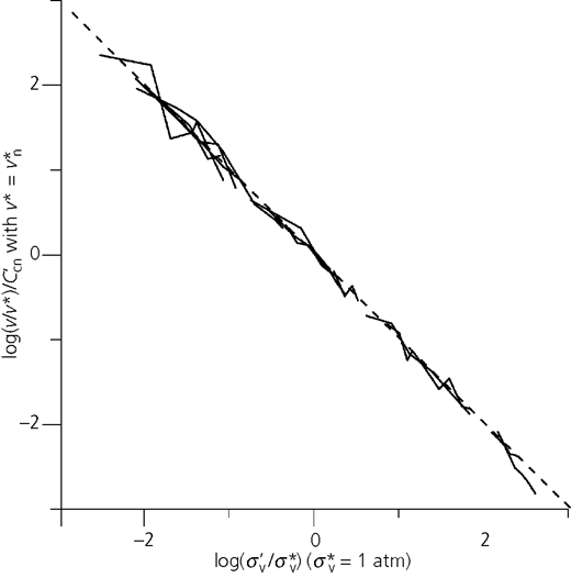
Since Equations 5 and 7 are merely normalised versions of the basic log(v) against equation with and or , it follows that a virgin compression line for any soil obeying Equation 1 can be normalised this way, generating a single, unique dimensionless compression line (ICL*) with a gradient = −1 passing through the coordinate origin.
This operation can be applied equally well to straight unloading lines in which is replaced by , where , the natural swelling index (Butterfield, 1979, 2011), is analogous to the swelling index C s associated with the , compression model.
If, however, the data either are or are considered to be a collection of individual points, there will be no means of estimating as done earlier. In this case, estimation of can be resorted to for each data point from their v L values and Equation 6, as Burland (1990) and Skempton (1970) did.
In Figure 7, the best-fit line through the data, the corresponding SCL* (SCL in the model) is shown dashed, together with the previously derived ICL*. The equation to the SCL* is
in which log(S) = 0·6 is the spacing between the two lines parallel to either axis.
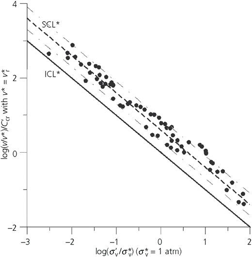
Complete natural-clay data set normalised by plotting against : the best-fit line through the data, the SCL* is shown as a dashed line, together with the previously derived ICL*
Complete natural-clay data set normalised by plotting against : the best-fit line through the data, the SCL* is shown as a dashed line, together with the previously derived ICL*
This figure is therefore an alternative means of comparing the compressibility of the natural and reconstituted soils to that shown in Burland’s, based (Figure 4), interpretation.
The actual gradient of the best-fit line through the points is −0·98 (R 2 = 0·963) which, within the precision of the data, confirms that the two lines are parallel with a gradient of −1. Hence, when the values of the normalised expressions for the natural soil and a reconstituted sample of it are equal, the ratio of their effective overburdens is
or
a ratio rather lower than Burland’s (1990) approximation of 5.
Practical implications
Since the model is equally valid for unloading processes in an oedometer (with replaced by ), a similar analysis could also generate information applicable to this situation.
The spacing of the lines predicts that at a given value of the logarithmic equivalent of the void index (Iv), the effective overburden carried by the natural clay is four times that carried by an equivalent reconstituted clay, rather than the fives times predicted by Burland (1990).
The complete model also provides an alternative, practically useful, interpretation of the preceding statement. Differentiating Equation 1 provides an expression for the ‘coefficient of volume compressibility’ in terms of at any point along a virgin compression line as
Therefore, a logarithmic plot of log(mv) against will have a gradient of −1 and a log(mv) intercept of .
A key component of the model (Butterfield, 2011) is that if a soil sample on the line is unloaded from to any point along a ‘swelling line’ and then reloaded back to , it will always lie on a line parallel to Equation 10 but with intercept .
Consequently, the spacing of the original and final load points parallel to the log(mv) axis will always be
Therefore, if mvr represents the local compressibility of a virgin (reconstituted) sample and mvn that of an identical natural sample which has been unloaded and reloaded as done earlier, the latter will have a compressibility rather than .
The assumption being made here is that the natural-clay sample will inevitably have undergone at least one modest in situ unload–reload cycle, due to wave action on a beach, for example, during and after deposition and thereby become less compressible. In his paper, Butterfield (2011) tabulated the ratios for 12 samples of seven different clays and silty clays; the average value of the ratios was 0·596, essentially identical to log(S), from which one might conclude that provides the ratio of the value of mv for a reconstituted marine clay sample to that of a natural in situ one, as in Figure 7, and an explanation of S.
Concluding remarks
The model of soil compressibility provides an alternative version of the ICL and SCL proposed by Burland (1990), in which both lines become straight and parallel, with a gradient of −1, when applied to Skempton’s (1970) data on ‘normally’ consolidated marine clays.
That the natural clays are stiffer than reconstituted, normally consolidated samples of the same soil by a factor of log10(4) is explained by the fact that this is the ratio expected for a soil that has been unloaded and reloaded to its present in situ effective stress if it has behaved as predicted by the extended log(v) against model of soil response in an oedometer. The marine deposits have therefore historically undergone, at least small, unload–reload cycles either during, or after, deposition: they are, in fact, not normally consolidated.