
A three-dimensional limit analysis of slopes is presented in this paper, based on a right circular cone failure surface. The associated translational mechanism appears to yield better assessment of the safety in isotropic rock than the traditional wedge-type mechanism. The strength of a bonded geomaterial was described using a linear strength envelope truncated in the tensile regime. The tensile strength cut-off so introduced constitutes a non-linear portion of the strength envelope, and it allows constructing failure mechanisms that include rupture modes, in addition to the shear deformation mode. Consequently, the mechanisms in materials with tension cut-off are more critical than those in materials with a traditional linear strength envelope. It is also demonstrated that the failure mechanism based on the right circular cone failure surface in vertical slopes yields results as good as or better than the more complex rotational mechanisms, although the difference is not very significant.
Notation
- A
area
- B
width of the mechanism
- b
width of plane insert
- c
intercept of linear portion of strength envelope
- D
rate of work dissipation in the mechanism
- d
rate of work dissipation per unit area of failure surface
- F
stability factor γ H/c or γ H/s u
- fc
uniaxial compressive strength
- ft
uniaxial tensile strength
- H
slope height
- L
length
- rO
radius of the failure surface at x = 0
- ri
radius of the i-segment of the failure surface
- su
undrained shear strength
- V
volume
- v
velocity vector
- Wγ
work rate of gravity forces
- x, y, z
Cartesian coordinates
- αi
inclination of segment i of the failure surface
- β
slope inclination angle
- γ
unit weight of geomaterial
- δ
rupture angle
- ζ
angle defining location of cone apex
- ηi
angle defining segment i
- θ
angle describing a portion of the cone embedded in soil
- λ
half-angle between two failure planes in wedge mechanism
- ξ
tensile strength fraction
- σ1, σ2, σ3
principal stresses
- φ
angle of internal friction
- χ
angle between velocity vector and the cross-section of failure planes in wedge mechanism
Introduction
The stability of rock and soil slopes has been considered by many, but the subject of three-dimensional (3D) limit analysis of slopes has received less attention. The slope material considered in this paper is a bonded geomaterial, such as bonded soils or soft rocks. While the strength criteria for such materials are typically non-linear in the first invariant of the stress tensor (Hoek and Brown, 1980; Hoek et al., 2002), they are often linearised in the analyses to resemble the traditional Mohr–Coulomb (M-C) function. For bonded geomaterials, the M-C function exhibits uniaxial tensile strength and even larger isotropic tensile strength. The significant difference in the analysis in this paper from the previous analyses, however, is the consideration of a limit on the tensile strength by introducing a tensile strength cut-off.
The description of observations of slope failures are found in the literature as early as 1846 (Collin, 1846), while the early engineering analyses of safety were developed in the early twentieth century (Fellenius, 1927; Taylor, 1937). Traditional analyses of assessment of slope safety typically include the plane strain assumption and a simplified method of calculations based on a global equilibrium of collapsing blocks. The latter is often referred to as the limit equilibrium method. Three-dimensional considerations are not common, not only because of the analytical complexity, but also because the two-dimensional (2D) analyses are more conservative in the assessments of safety. However, in cases such as excavations or when the slope is physically restrained by a harder rock outcrop, a 3D analysis may be called for.
The early 3D analyses included techniques that were generalisations of the popular ‘slice techniques’ to include ‘columns’ as primary blocks (Hovland, 1977; Hungr, 1987), without much consideration given to kinematics. The latter was only considered in the presumed shape of the failure mechanism, but the analyses did not assure the admissibility of the mechanisms from the standpoint of plastic flow. While the kinematic approach of limit analysis did provide admissible 3D mechanisms, these mechanisms were first restricted to rigid block translation (Drescher, 1983; Michalowski, 1989), because of the complexity in generalising the 2D rotational failures (Chen, 1975; Drucker and Prager, 1952) to 3D geometries. The exceptions were undrained failures, where any surface of revolution constitutes an admissible failure surface (Baligh and Azzouz, 1975; Gens et al., 1988). Rotational 3D failures were then considered for pressure-dependent materials using the limit equilibrium technique (Leshchinsky et al., 1985) and kinematic limit analysis (De Buhan and Garnier, 1998; Michalowski, 2010; Michalowski and Drescher, 2009). Numerical approaches, typically based on finite-element analysis, have also been carried out in the last decades (Griffiths and Marquez, 2007; Li et al., 2010).
A common failure mechanism considered in rock slope engineering is a wedge collapse (e.g. Goodman, 1993; Hoek and Bray, 1981). The planes of failure may be defined by the distribution of joints in the rock, and weathered rocks might also display wedge-type failures. Wedge-type analyses consider purely translational kinematics limited to one sliding block. Considerations of this kind, based on the limit equilibrium technique, can be found, for example, in the book by Hoek and Bray (1981). An equally reasonable mechanism in soils and weathered rocks is a translational collapse with the failing block defined by the surface of a cone rather than a wedge. Preliminary analyses in isotropic geomaterials indicated that a translational movement of a block defined by a conical surface is a more critical mechanism than a wedge-type translation. Such a mechanism of failure is considered in this paper, with additional modification, which limits the tensile strength of the geomaterial. The novelty in this paper is in demonstrating a conical mechanism of slope failure in geomaterial with tensile strength cut-off and in presenting a stability analysis that includes tension cut-off.
The concept of tension cut-off modification is described first. Next, a simple wedge mechanism and a conical mechanism of slope failure are considered in an M-C geomaterial, followed by a demonstration that a right circular cone mechanism provides more critical results. Finally, the analysis of the slope failure based on a right circular cone failure surface in the material with tension cut-off is described.
Tensile strength cut-off
Bonded geomaterials are characterised by both uniaxial compressive strength and tensile strength. While the tensile strength of rocks is a matter of routine testing, strength of hard (bonded) soils is typically tested in a compressive regime. The tensile strength is then arrived at as an extrapolation of the test results into the tensile regime. Consequently, the material is described by the M-C strength envelope with uniaxial tensile strength and even larger triaxial (isotropic) tensile strength. Drucker and Prager (1952) recommended eliminating the tensile strength from the strength criterion for geomaterials, while Paul (1961) suggested introducing a tensile strength cut-off as a fracture criterion for brittle geomaterials. The tensile strength cut-off can reduce the uniaxial tensile strength when compared to that in the classical M-C function, or it can eliminate the tensile strength altogether, as suggested by Drucker and Prager (1952).
Figure 1(a) illustrates an M-C failure surface with Paul’s tension cut-off modification in the principal (Haigh–Westergaard) stress space. Elastic stresses in the tensile regime are limited with three mutually perpendicular planes, as illustrated in Figure 1(a). This is essentially the Galileo–Rankine tensile strength criterion (Lagioia et al., 2014). The associativity of the plastic flow enforced in the limit analysis renders the strain rate vector perpendicular to the failure surface, but the vector normal to the surface is not unique along the edges where the three planes intersect with one another – for example, AF and FE (or with the M-C surface, AB) – or along the meridians of the surface (e.g. AD and BC). The transformation of the stress state from the Haigh–Westergaard space onto the Mohr plane is shown in Figure 1(b). If convention is assumed, then plane ABCD in the principal stress space relates to the linear portion of the strength envelope, whereas plane ABEF contains all admissible stress states with . For instance, at point F, (isotropic tension), whereas at point G, (uniaxial tension). These two stress states map onto Figure 1(b) as a Mohr circle reduced to a point at and a Mohr circle with diameter ft (marked in Figure 1(b)), respectively.
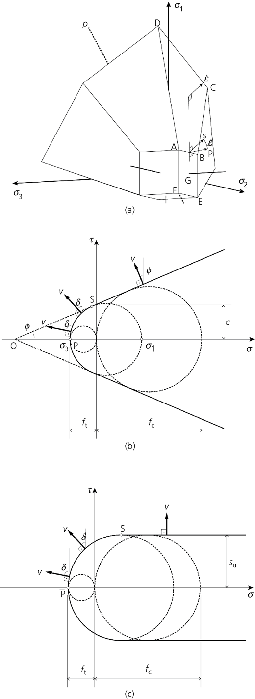
Tensile strength cut-off: (a) yield surface in the principal stress space suggested by Paul (1961), (b) strength envelope and (c) strength envelope for undrained process
Tensile strength cut-off: (a) yield surface in the principal stress space suggested by Paul (1961), (b) strength envelope and (c) strength envelope for undrained process
The authors will define the strength of the geomaterial with tension cut-off with three parameters: uniaxial compressive strength fc, uniaxial tensile strength ft and internal friction angle φ. The rate of work dissipation per unit area of a failure surface governed by the tension cut-off and the normality flow rule can be written as (Michalowski, 1985)
where v is the magnitude of kinematic discontinuity vector v, and angle δ is indicated in Figure 1(b). Eliminating tension cut-off from the strength envelope by setting δ = φ, the well-known dissipation rate expression for the M-C strength criterion follows (e.g. Chen, 1975)
From the standpoint of plasticity theory, angle δ describes the volumetric deformation, but it is not a dilatancy angle in the Reynolds (1885) sense. Pressure-dependent materials, including geomaterials, exhibit dilatancy that is typically significantly lower than that produced by the normality flow rule. Nevertheless, it can be proved that the limit analysis solution based on a mechanism conforming to the normality flow rule yields a rigorous bound to the true solution (Radenkovic, 1962), even if the true dilatancy rate is lower than that following from the normality flow rule. In order to avoid any confusion, angle δ will be referred to as the rupture angle, which is consistent with Paul’s (1961) intention of using the tension cut-off as a fracture criterion. Not surprisingly, the tension cut-off was found to be useful in describing slope failure mechanisms with opening cracks as part of the collapse process (Michalowski, 2013).
Consider now an undrained plastic deformation in a saturated porous material. Under undrained conditions, deformation is incompressible, but a rupture of the material associated with cavitation in water is possible, particularly if bubbles of air are present in the pore water. The strength envelope for a material during undrained deformation is illustrated in Figure 1(c), with the curvilinear portion associated with the rupture of the material. The rate of work dissipation per unit area of a failure surface subjected to rupture now becomes
with su being the undrained shear strength in the compressive regime. For the linear portion of the strength envelope, the rate of the work dissipation per unit area reduces to
While the deformation associated with the curvilinear portion of the strength envelope can no longer be interpreted as continual strain, the mechanism of incipient failure with some portions subjected to rupture is a legitimate mechanism that can be used in the limit analysis to calculate the loads associated with incipient failure.
Geotechnical stability analyses in geomaterials with tension cut-off were presented recently in both plane–strain analyses (Michalowski, 2017, 2018) and analyses with 3D failure geometry (Park and Michalowski, 2017). The outcome of these analyses indicates that tension cut-off can have a very significant effect on the outcome of the stability analyses. In this paper, a specific mechanism of slope failure is considered, based on a right circular cone failure surface.
Problem statement and the method of analysis
A slope of height H is given with a unique inclination angle β and unit weight γ. The width of the mechanism is limited to some value B. The soil/rock strength is defined by the M-C criterion with or without a tensile strength cut-off. The parameters characterising the strength are the uniaxial compressive strength fc, uniaxial tensile strength ft (bonded geomaterial) and internal friction angle φ. Given the stress-free boundary of the slope, determine stability factor F
which defines the combination of the slope parameters when the slope is at the verge of failure. Parameter c is uniquely related to the uniaxial compressive strength and the internal friction angle
and it is the M-C function intercept on the ordinate on the Mohr plane; depending on the tensile strength, parameter c may or may not be equal to cohesion for a bonded geomaterial. For the classical M-C medium, the uniaxial tensile strength is uniquely related to the uniaxial compressive strength
Hence, the M-C criterion is a function of two material parameters, while the model with tension cut-off is a function of three material parameters.
The kinematic approach of limit analysis will be used, which requires that an admissible mechanism of failure is found first. Limit analysis yields rigorous bounds to limit loads or other measures of stability, here the stability factor in Equation 5. The admissibility of the mechanism requires that the kinematics be consistent with the normality rule of plastic flow and the boundary conditions of the problem. The former requires that vectors of velocity be inclined at the angle of internal friction to the shear failure surfaces or the angle of rupture at the surfaces governed by tension cut-off. The kinematic approach of limit analysis is based on the balance of work rate written for a given mechanism
where D is the rate of internal work in the entire mechanism during incipient failure (rate of dissipated work) and Wγ is the rate of work of external forces (here, weight). This approach yields the upper bound to the stability factor in Equation 5. The best solution is then obtained by minimising the upper bound with the geometry of the mechanism being varied.
First, a wedge mechanism and a cone mechanism are considered with strength represented by the M-C strength envelope, in order to indicate that in an isotropic material (no distinct joints), the cone mechanism yields a better (lower) estimate of the stability factor. As indicated earlier, the classical M-C function depends only on two out of three strength parameters: fc, ft and φ. Choosing the uniaxial compressive strength and the internal friction angle, the rate d of dissipated work per unit area of a failure surface in an M-C material can be written as
where v is the magnitude of the velocity jump vector v on the failure surface. Readers will notice that by using Equation 6, this dissipation rate will reduce to the classical expression (Drucker and Prager, 1952). Second, the tensile strength cut-off will be introduced, and the conical mechanism in a geomaterial with tension cut-off will be developed.
Wedge mechanism
Wedge-type mechanisms are commonly considered in the stability of rock slopes (e.g. Hoek and Bray (1981)), particularly in rocks with distinct sets of joints. Here, the wedge failure mechanism is considered in an isotropic medium, with strength determined by the classical M-C function where the tensile strength is uniquely related to the compressive strength (Equation 7). This mechanism is illustrated in Figure 2; it is revisited here in order to assess its effectiveness in isotropic formations when compared to a conical collapse mechanism. The wedge is formed by two planes: ACF and ACL. The kinematic admissibility requires that velocity vector v be inclined at φ to both planes; therefore, vector v must make some larger angle χ with line AC (this is because angle φ is the smallest angle between vector v and any line on either of the two planes). If the angle between the two planes of failure is 2λ, then, based on the geometry of the wedge (Figure 2(b)), one can find the relationship among angles λ, χ and φ
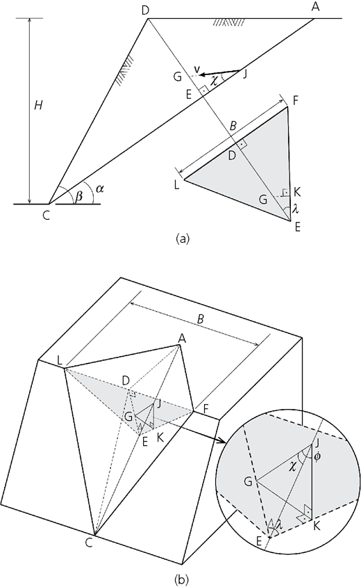
Considering the geometrical relations in Figure 2, one can easily find the two terms in the balance Equation 8, which leads to the following expression for the stability factor.
where angles χ and λ are defined in Equations 10 and 33, respectively. The steps leading to Equation 11 are shown in the Appendix.
In jointed rocks, the planes of failure are likely to coincide with the dominant joints, and the wedge does not need to be symmetric nor does the failure need to reach the toe. However, isotropic geomaterials are considered here, with limit B set on the maximum width of the mechanism, forcing the critical mechanism to reach the toe, unless the width of the slope is very small.
Right circular cone failure surface
The conical mechanism of slope failure in geomaterial described by the classical M-C function is illustrated in Figure 3. A right circular cone with apex angle 2φ constitutes an admissible failure surface in a rigid-block mechanism (φ is the internal friction angle). Curvilinear cones were explored in calculations of the bearing capacity of rectangular footings (Michalowski, 2001) and were later employed in 3D analyses of slope failure (Michalowski, 2010; Michalowski and Drescher, 2009). A cone with base radius rO intersects the slope, forming a single block moving with velocity v. The moving block is defined by the surface of the slope and a portion of the conical surface embedded in the slope. Cross-sections of the cone are illustrated by circles above and below the slope in Figure 3, with the shaded areas defining the rock/soil in the sliding block. The location of apex P of the cone is determined by angles α and ζ. Knowing that the cone apex angle is 2φ, the centre of the cone base O can be found and the radius of the base of the cone rO can be determined from the following relation
whereas the radius of an arbitrary cross-section depends on coordinate z
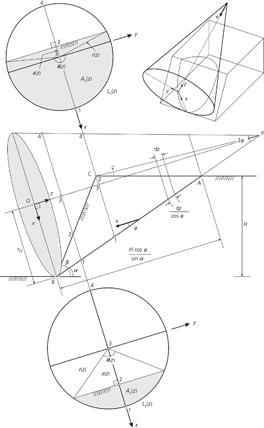
In order to integrate the rate of work dissipation (left side of Equation 8), the area of the interface of the moving block with the material at rest needs to be determined. An infinitesimal area element can be defined as
where Lc is the length of circular arc of the shaded segments indicated in Figure 3. Length Lc can be easily determined as
with r(z) in Equation 13 and angle θ calculated from Equation 37 in the Appendix. The rate of work dissipation per unit area of kinematic discontinuity in an M-C material is expressed in Equation 9; consequently, the total dissipation in Equation 8 can be calculated from the following expression.
With angle θ calculated in Equation 37, the area of the shaded portion Ac of the circular cross-section is given as
and the work rate of the material weight Wγ is
Consequently, using the balance in Equation 8 and the expression in Equation 6, the stability factor γ H/c is found as
Conical failure surface with an insert
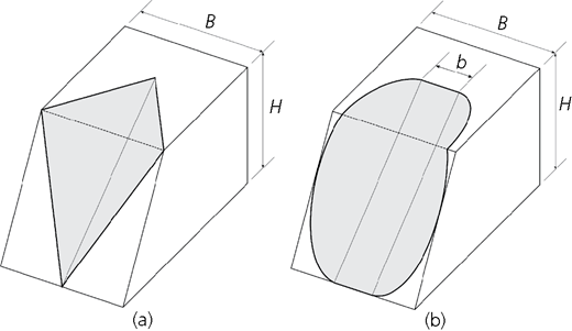
In order to make the mechanism realistic for long slopes, an insert of width b is introduced into the mechanism. Readers will notice that inserting a plane segment into the wedge mechanism in Figure 4(a) would constitute inadmissible kinematics as velocity vector v would be inclined at angle χ (rather than φ) to the plane of failure. However, a conical mechanism with a plane insert, as illustrated in Figure 4(b), is admissible. Including the contribution of the plane insert into the dissipation rate and the work rate of the material weight is straightforward, leading to
where L p is the length of distance AB in Figure 3 and A p is the area of triangle ABC.
In the case of undrained collapse, the strength is represented by undrained shear strength s u and the failure surface becomes a circular cylinder. The cross-section P of the lines inclined at α and at ς (Figure 3) now is not an apex, but an arbitrary point on the cylindrical surface. The authors now make an arbitrary assumption that the distance of that point from the horizontal surface of the slope is equal to r O
The calculations for undrained failures can now be carried out for undrained cases using the same algorithm, but the expression in Equation 12 needs to be replaced with that in Equation 21, while the internal friction is set to zero.
Calculated stability factors
Calculations have been carried out to compare the stability factors for the wedge and the conical mechanisms with a plane insert with the strength defined by the classical M-C function. The respective expressions for the two mechanisms are given in Equations 11 and 20. The width of the mechanism was limited by ratio B/H, with B being the limit set on the width of the mechanism. The solutions to the stability factor were minimised, as the kinematic approach leads to the upper bound on the stability factor. The parameter variable in the wedge mechanism was angle α, whereas angle λ was determined by width B of the mechanism (Figure 2). In the conical mechanism, angles α and ζ were variable (Figure 3). Calculations were carried out in repeated loops with angles varied by an increment of 0·01°. Computations were stopped when the difference between two consecutive stability factors was smaller than 10−6. The numerical outcome is illustrated in Figure 5. Stability factors are shown for undrained failure and for an internal friction angle up to 30°, and for ratio B/H varied from 0·5 to 5; for comparison, a plane case is also presented.
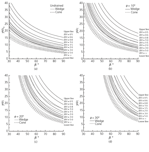
Comparison of stability factors for the wedge and cone mechanisms in an M-C material: (a) undrained failure process; (b) drained process, φ = 10°; (c) φ = 20°; and (d) φ = 30°
Comparison of stability factors for the wedge and cone mechanisms in an M-C material: (a) undrained failure process; (b) drained process, φ = 10°; (c) φ = 20°; and (d) φ = 30°
The calculations reveal that in all cases, the solution with the cone mechanism is better (lower) than that based on the wedge mechanism. For example, for a narrow slope with B/H = 0·5, the stability factor for undrained wedge failure in a 45° slope is 59% larger than the stability factor based on the conical mechanism. This difference drops to 43% for a failure width B/H = 5. In the material with an internal friction angle of 30°, the respective differences for a 45° slope are 57% and 46%. The trend is somewhat different for a vertical slope; when φ = 30°, the difference is 31% for a narrow slope (B/H = 0·5) and 44% for a wide slope (B/H = 5). More comprehensive numerical results for the undrained failure are included in Table 1 and in Table 2 for φ = 30°.
Stability factors γ H/s u for undrained failure of slopes
| B/H | Mechanism | Slope inclination angle β | ||||
|---|---|---|---|---|---|---|
| 30° | 45° | 60° | 75° | 90° | ||
| 0·5 | Wedgea | 42·85 | 28·79 | 21·88 | 17·87 | 15·36 |
| M-Cb | 27·15 | 18·07 | 13·54 | 10·86 | 9·17 | |
| T-Cc | 25·27 | 16·67 | 12·39 | 9·93 | 8·48 | |
| 0·6 | Wedgea | 38·58 | 25·81 | 19·50 | 15·79 | 13·44 |
| M-Cb | 24·98 | 16·56 | 12·34 | 9·80 | 8·14 | |
| T-Cc | 23·02 | 15·10 | 11·13 | 8·72 | 7·27 | |
| 0·8 | Wedgea | 33·35 | 22·16 | 16·57 | 13·24 | 11·07 |
| M-Cb | 22·31 | 14·71 | 10·87 | 8·54 | 6·97 | |
| T-Cc | 20·23 | 13·18 | 9·58 | 7·38 | 5·89 | |
| 1 | Wedgea | 30·32 | 20·05 | 14·88 | 11·76 | 9·70 |
| M-Cb | 20·74 | 13·63 | 10·02 | 7·81 | 6·30 | |
| T-Cc | 18·58 | 12·04 | 8·69 | 6·60 | 5·15 | |
| 1·5 | Wedgea | 26·59 | 17·43 | 12·78 | 9·93 | 8·00 |
| M-Cb | 18·71 | 12·23 | 8·92 | 6·88 | 5·46 | |
| T-Cc | 16·42 | 10·57 | 7·54 | 5·62 | 4·25 | |
| 2 | Wedgea | 24·96 | 16·29 | 11·86 | 9·12 | 7·24 |
| M-Cb | 17·72 | 11·55 | 8·39 | 6·43 | 5·07 | |
| T-Cc | 15·36 | 9·84 | 7·00 | 5·19 | 3·84 | |
| 3 | Wedgea | 23·62 | 15·35 | 11·10 | 8·45 | 6·60 |
| M-Cb | 16·75 | 10·89 | 7·88 | 6·00 | 4·69 | |
| T-Cc | 14·31 | 9·13 | 6·47 | 4·77 | 3·48 | |
| 5 | Wedgea | 22·85 | 14·81 | 10·66 | 8·05 | 6·23 |
| M-Cb | 16·00 | 10·38 | 7·48 | 5·67 | 4·40 | |
| T-Cc | 13·49 | 8·60 | 6·06 | 4·44 | 3·23 | |
| 2D | M-Cb | 14·92 | 9·65 | 6·92 | 5·21 | 4·00 |
| T-Cc | 12·24 | 7·78 | 5·46 | 3·97 | 2·88 | |
Wedge mechanism
Right circular cone mechanism and M-C strength envelope
Right circular cone mechanism with tension cut-off strength envelope
Stability factors γ H/c for slopes in geomaterial with φ = 30°
| B/H | Mechanism | Slope inclination angle β | |||
|---|---|---|---|---|---|
| 45° | 60° | 75° | 90° | ||
| 0·5 | Wedgea | 190·75 | 68·34 | 38·88 | 26·62 |
| M-Cb | 121·81 | 46·51 | 27·71 | 20·24 | |
| T-Cc | 119·84 | 45·31 | 26·85 | 19·24d | |
| 0·6 | Wedgea | 172·20 | 60·87 | 34·31 | 23·27 |
| M-Cb | 108·38 | 39·45 | 23·72 | 16·34 | |
| T-Cc | 105·52 | 37·68 | 21·68 | 15·18d | |
| 0·8 | Wedgea | 150·01 | 51·82 | 28·74 | 19·18 |
| M-Cb | 95·74 | 33·17 | 18·49 | 12·43 | |
| T-Cc | 92·52 | 31·16 | 16·89 | 11·28 | |
| 1 | Wedgea | 137·58 | 46·66 | 25·54 | 16·81 |
| M-Cb | 89·51 | 30·28 | 16·58 | 10·89 | |
| T-Cc | 85·98 | 28·20 | 14·90 | 9·39 | |
| 1·5 | Wedgea | 122·89 | 40·40 | 21·59 | 13·85 |
| M-Cb | 82·50 | 27·07 | 14·46 | 9·24 | |
| T-Cc | 78·47 | 24·78 | 12·69 | 7·69 | |
| 2 | Wedgea | 116·82 | 37·72 | 19·87 | 12·54 |
| M-Cb | 79·47 | 25·79 | 13·56 | 8·55 | |
| T-Cc | 75·17 | 23·29 | 11·72 | 6·88 | |
| 3 | Wedgea | 112·02 | 35·55 | 18·45 | 11·44 |
| M-Cb | 76·87 | 24·53 | 12·77 | 7·94 | |
| T-Cc | 72·14 | 21·94 | 10·85 | 6·21 | |
| 5 | Wedgea | 109·38 | 34·32 | 17·63 | 10·79 |
| M-Cb | 74·68 | 23·59 | 12·19 | 7·50 | |
| T-Cc | 69·89 | 20·94 | 10·22 | 5·71 | |
| 2D | M-Cb | 71·88 | 22·39 | 11·42 | 6·92 |
| T-Cc | 66·76 | 19·57 | 9·35 | 5·12 | |
Wedge mechanism
Right circular cone mechanism and M-C strength envelope
Right circular cone mechanism with tension cut-off strength envelope
Face failure mechanism
Cone failure surface in geomaterials with tension cut-off
Consider now a slope in a material with strength described by the envelope in Figure 1(b). The failure mechanism includes only one block moving with velocity v, but the failure surface can be inclined to velocity v at angle δ spanning from φ to 90°, as determined by the plastic flow rule associated with section SP of the strength envelope in Figure 1(b). Angle δ is not the dilatancy angle in the Reynolds (1885) sense; rather, it relates to discontinuous deformation with a large separation component, and it was termed a rupture angle earlier (Park and Michalowski, 2017).
A schematic diagram of construction of the failure mechanism is illustrated in Figure 6. Points B1,…,Bi,…,Bn and Bn+1 on the failure surface are determined by variable angles ηi and αi (i = 1, 2,…,n). Points B1,…,Bi,….,Bn, Bn+1, C, B1 determine a cross-section of a single block moving with velocity v. Each of n segments Bi – Bi+1 (i = 1, 2,…,n) along the trace of the failure surface in Figure 6(a) constitutes a segment of a generatrix of a cone with apex at Pi and apex angle equal to 2δi, with δ1 = φ. The inclination α1 of the first segment determines the direction of the block velocity v (inclined at φ to segment B1 – B2). Once all angles αi are selected, the rupture angle δi at all remaining segments are determined from the following expression
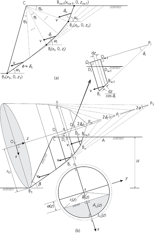
Multicone failure mechanism in geomaterial with tension cut-off: (a) central cross-section of the moving block and (b) mechanism construction details
Multicone failure mechanism in geomaterial with tension cut-off: (a) central cross-section of the moving block and (b) mechanism construction details
Readers will notice that the rupture angles δi on all segments are uniquely related to the geometry of the mechanism; hence, they are determined in the process of optimisation of the mechanism when the minimum of the stability factor is sought. While the rupture angle varies from one segment of the failure surface to the next, the material is homogeneous, and it can assume any rupture angle between φ and 90° at any point within the slope.
The geometry of the entire mechanism is determined by n angles αi and n − 1 angles ηi. Each of points Bi has coordinates xi, 0 and zi, easily calculated for given angles αi and ηi. Radius ri(z) of cone i with generatrix Bi – Bi + 1 is determined from the expression
Length Lci marked in Figure 6 can be calculated as
where θi(z) is calculated from Equation 40. Considering the rate of work dissipation per unit area in Equation 1, the dissipation integrated over the entire failure surface becomes
The summation in Equation 25 is over n conical segments with various angles δi, whereas the integration takes place over the surfaces within individual segments. The shaded area Aci in Figure 6 is
and the rate of work of the material weight becomes
Using the work rate balance in Equation 8, one arrives at the following expression for the stability factor of a slope built of geomaterial with tension cut-off
To simplify the expression for the stability factor, parameter ξ was introduced, which represents the uniaxial tensile strength ft as a function of the uniaxial compressive strength
Coefficient ξ can vary from 0 to 1; at value 1, the tensile strength ft becomes equal to that in the M-C function (Equation 7).
Conical failure mechanism with tension cut-off and an insert
In order to allow the stability factor to approach that for a 2D mechanism for large B/H ratios, a plane portion was inserted into the mechanism similar to that illustrated in Figure 4(b), but with multiple sections in the rupture zone, consistent with the mechanism in Figure 6(b). With b being the width of the plane insert and L pi and A pi being the length of segment Bi – Bi+1 and area of triangle CBiBi+1, respectively (Figure 6(a)), the stability factor for the conical mechanism with plane insert takes the form
Calculated stability factors for geomaterials with tension cut-off
Calculations were carried out for slopes with an inclination angle ranging from 30° to 90°, for an internal friction angle up to 30° and for undrained failure. The mechanism with n segments is defined by angle ζ, n angles αi and n − 1 angles ηi. The stability factor in Equation 30 was minimised with angles ζ, αi and ηi being variable. All angles were varied in repeated loops, with a minimum increment of 0·01°, until the difference between two consecutive stability factors was less than 10−6. The number of segments of the moving block was chosen based on the initial analysis of the dependence of the calculated stability factor on the number of segments. The outcome of this analysis is illustrated in Figure 7. The calculation for one segment (n = 1) includes only the classical M-C material strength. The drop in the stability factor is the largest when the number of segments is increased to 2. Subsequently, the addition of one segment produces a progressively smaller improvement in the solution, with no benefit in increasing the number of segments beyond ten. Consequently, all calculations were performed for ten segments. The relative difference at the bottom of Figure 7 indicates the difference between two consecutive solutions for n and n + 1 blocks.
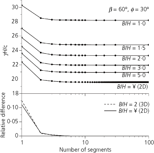
Dependence of the calculated stability factor on the number of conical segments in the moving block and relative difference between two consecutive solutions for n and n + 1 blocks
Dependence of the calculated stability factor on the number of conical segments in the moving block and relative difference between two consecutive solutions for n and n + 1 blocks
The comparison of the stability factors for the slope in the geomaterial with full tension cut-off ( f t = 0 or ξ = 0) to those from a more traditional M-C analysis is illustrated in Figure 8. The solutions are presented for the undrained process of failure and for geomaterial with an internal friction angle up to 30°. It is not surprising that in all cases, the consideration of tension cut-off yields a better (lower) solution to the stability factors than the analyses based on the traditional M-C strength. Numerical values of the stability factors are included in Tables 1 and 2. The largest difference was found for an undrained failure process. This difference for the narrow slopes (B/H = 0·5) is about 7%, independent of the slope inclination, but it increases for wider slopes; for wider slopes, this difference becomes dependent on the inclination. For example, for undrained failure and B/H = 5, the difference is 16% for a gentle slope with an inclination angle of 30° and 27% for a vertical slope. When φ = 30°, the respective differences are 6 and 24%.
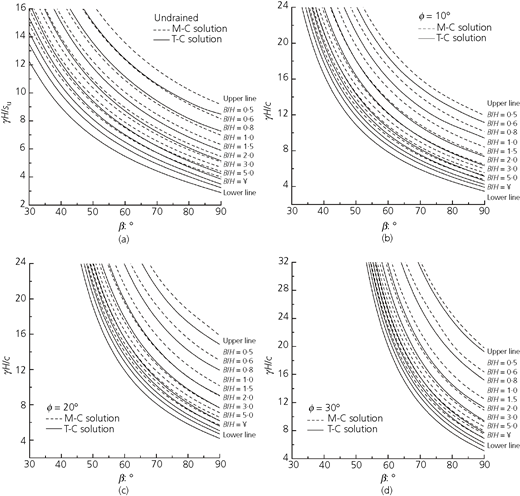
Comparison of stability factors for the conical block mechanism without tension cut-off (M-C) and with tension cut-off (T-C, zero tensile strength ξ = 0): (a) undrained failure process; (b) drained process, φ = 10°; (c) φ = 20°; and (d) φ = 30°
Comparison of stability factors for the conical block mechanism without tension cut-off (M-C) and with tension cut-off (T-C, zero tensile strength ξ = 0): (a) undrained failure process; (b) drained process, φ = 10°; (c) φ = 20°; and (d) φ = 30°
It is interesting to compare the current results to the outcome of the 3D analysis with a rotational failure mechanism. This mechanism includes a curvilinear conical surface (or a horn-like surface) and was described in a paper by Michalowski and Drescher (2009). More recently, this mechanism was generalised to include the tension cut-off; the reader will find more details regarding this mechanism in the paper by Park and Michalowski (2017). When calculations of the stability factor consider geomaterial with strength governed by the M-C function, the rotational mechanism appears to be more critical than the translational mechanism based on a right circular cone. However, when tensile strength cut-off is considered, the latter can yield better (lower) stability factors for vertical slopes, although the difference is small and probably negligible from a practical standpoint. This is demonstrated by the results in Table 3. For narrow slopes, the most critical mechanisms were found not to reach the toe of the slope (face failure mechanisms).
Stability factors γ H/s u and γ H/c for vertical slopes in geomaterials with tension cut-off (ξ = 0)
| B/H | Undrained | φ = 30° | ||
|---|---|---|---|---|
| Translational mechanisma | Rotational mechanismb | Translational mechanisma | Rotational mechanismb | |
| 0·5 | 8·48 | 8·42c | 19·24c | 18·34c |
| 0·6 | 7·27 | 7·27 | 15·18c | 15·10c |
| 0·8 | 5·89 | 6·03 | 11·28 | 11·11 |
| 1 | 5·15 | 5·27 | 9·39 | 9·46 |
| 1·5 | 4·25 | 4·38 | 7·69 | 7·62 |
| 2 | 3·84 | 3·91 | 6·88 | 6·91 |
| 3 | 3·48 | 3·54 | 6·21 | 6·24 |
| 5 | 3·23 | 3·27 | 5·71 | 5·78 |
| 2D | 2·88 | 2·92 | 5·12 | 5·19 |
Right circular cone surface
Curvilinear cone surface (Park and Michalowski, 2017)
Face failure mechanism
Calculations carried out with a seismic load (defined by a coefficient of horizontal acceleration k h and considered in the analysis as a quasi-static force) indicated that the translational mechanism consistent with a right circular cone surface becomes more critical as the intensity of the seismic load increases. This is illustrated in Figure 9 for vertical slopes, for both the undrained slope failure and the drained failure in a material with φ = 30°. Material with full tension cut off (ξ = 0) was considered in both the rotational and translational analyses. Numerical results for vertical slopes are presented in Table 4. The differences between the results of the two analyses are, again, small. However, the mechanism based on a right circular cone surface appears to be quite competitive for vertical slopes when compared to the much more complex rotational mechanism (Park and Michalowski, 2017).
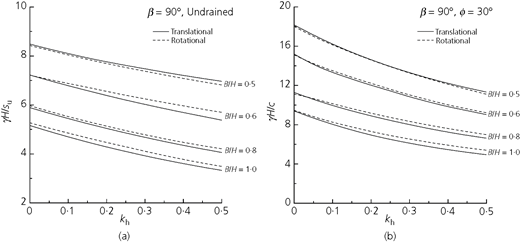
Stability factors for vertical slopes with tension cut-off as a function of seismic coefficient k h: (a) undrained failure and (b) failure in a material with φ = 30°
Stability factors for vertical slopes with tension cut-off as a function of seismic coefficient k h: (a) undrained failure and (b) failure in a material with φ = 30°
Stability factors γ H/s u and γ H/c for vertical slopes subjected to seismic acceleration in geomaterial with tension cut-off (ξ = 0)
| B/H | Seismic acceleration, k h | Undrained | φ = 30° | ||
|---|---|---|---|---|---|
| Translational mechanisma | Rotational mechanismb | Translational mechanisma | Rotational mechanismb | ||
| 0·5 | 0·1 | 8·10 | 8·04c | 16·20c | 16·12c |
| 0·3 | 7·47c | 7·37c | 13·29c | 13·26c | |
| 0·5 | 6·97c | 6·81c | 11·32c | 11·10c | |
| 0·6 | 0·1 | 6·79 | 6·87 | 13·31c | 13·49c |
| 0·3 | 6·02 | 6·24 | 10·82c | 11·01c | |
| 0·5 | 5·38c | 5·69 | 9·02c | 9·21c | |
| 0·8 | 0·1 | 5·44 | 5·52 | 9·94c | 10·13 |
| 0·3 | 4·67 | 4·78 | 8·01c | 8·33c | |
| 0·5 | 4·06 | 4·20 | 6·62c | 6·98c | |
| 1 | 0·1 | 4·69 | 4·84 | 8·02c | 8·24 |
| 0·3 | 3·92 | 4·10 | 6·10c | 6·54 | |
| 0·5 | 3·33 | 3·48 | 4·93c | 5·39 | |
Right circular cone surface
Curvilinear cone surface (Park and Michalowski, 2017)
Face failure mechanism
To facilitate readers in carrying out their own computations, four example solutions are presented with detailed outcomes regarding the geometry of the critical mechanisms. These examples are illustrated in Figure 10. All these examples were calculated using five segments in the mechanism (n = 5), each segment described with individual angles αi and ηi (i = 1, 2,…, 5), as illustrated in Figure 6(a). The search for the critical mechanisms was carried out with variable angles αi and ηi (and angle ς) with the smallest increment of 1°. Once the minimum stability factor is found, the angles associated with that minimum describe the geometry of the critical mechanism. The respective values of these angles for the two mechanisms with undrained collapse are included in Table 5, whereas for the drained failure, they can be found in Table 6.
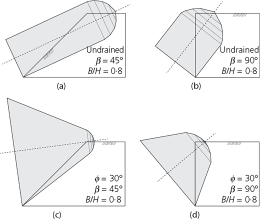
Critical mechanisms for example solutions with tension cut-off: (a) undrained failure of a 45° slope, (b) undrained failure of a vertical slope, (c) drained failure of a 45° slope and (d) drained failure of a vertical slope
Critical mechanisms for example solutions with tension cut-off: (a) undrained failure of a 45° slope, (b) undrained failure of a vertical slope, (c) drained failure of a 45° slope and (d) drained failure of a vertical slope
Example solutions for undrained collapse with tension cut-off (ξ = 0): five segments, B/H = 0·8
| β: ° | b/H | Critical mechanism variables: ° | γ H/s u | ||||||||||
|---|---|---|---|---|---|---|---|---|---|---|---|---|---|
| ς | α 1 | α 2 | α 3 | α 4 | α 5 | η 1 | η 2 | η 3 | η 4 | η 5 | |||
| 45 | 0·15 | 10 | 25 | 38 | 58 | 77 | 94 | 79 | 13 | 15 | 13 | 15 | 13·25 |
| 90 | 0 | 20 | 52 | 75 | 90 | 100 | 118 | 40 | 6 | 10 | 10 | 24 | 5·92 |
Examples solutions for drained collapse with tension cut-off (ξ = 0): φ = 30°: five segments, B/H = 0·8
| β: ° | b/H | Critical mechanism variables: ° | γ H/c | ||||||||||
|---|---|---|---|---|---|---|---|---|---|---|---|---|---|
| ς | α 1 | α 2 | α 3 | α 4 | α 5 | η 1 | η 2 | η 3 | η 4 | η 5 | |||
| 45 | 0·18 | 8 | 38 | 53 | 66 | 79 | 89 | 62 | 17 | 19 | 19 | 18 | 92·74 |
| 90 | 0 | 29 | 70 | 93 | 110 | 118 | 123 | 38 | 15 | 15 | 7 | 15 | 11·40 |
All examples are for relatively narrow slopes of B/H = 0·8, and it is interesting to notice that the critical mechanisms for the 45° slopes include a small 2D insert, as indicated in Tables 5 and 6 (and illustrated schematically in Figure 4(b)), whereas the critical mechanisms for the vertical slopes do not include an insert. The reader will notice that the stability factors calculated (last columns in Tables 5 and 6 differ only slightly from those in Tables 1 and 2 for the tension cut-off solutions. This difference is owed to the smaller number of mechanism segments in the calculations (5 against 10) and the coarser angle increment (1° against 0·01°) in the search for the critical mechanism.
Conclusions
Most traditional analyses of assessment of slope stability are 2D and use the classical M-C strength envelope. The analysis presented in this paper includes a mechanism with 3D geometry and a material whose strength is truncated in the tensile range, which leads to a non-linear strength envelope in the low-stress regime. Such a model is applicable for geomaterials with bonded grains, such as soft rocks and hard soils. The specific failure mechanism considered in this paper is based on a right circular cone failure surface. It was demonstrated that in isotropic soil or rock, such a mechanism produces a considerably better outcome (lower stability factors) than the wedge mechanism commonly used in rock engineering.
A tension cut-off, although suggested earlier in geomechanics, was only recently applied to safety assessment of slopes. The non-linearity in the strength envelope owed to truncation of tensile strength increases the multiplicity of admissible failure mechanisms that can be constructed. This is because the non-linearity allows failure modes typical of brittle materials, such as rupture and separation. This is consistent with a slope failure mode, such as toppling, where the blocks of bonded soil or rock separate. It was demonstrated that the slopes in geomaterial with tension cut-off are more vulnerable to failure than those in the material described with the traditional M-C yield condition (all other parameters the same). It was also demonstrated that for vertical slopes, the single-block translational mechanism with a right circular failure surface is competitive with the more elaborate rotational mechanism using a curvilinear cone failure surface.


Appendix
Wedge mechanism
It is presumed that toe failure occurs; hence, there is a unique relationship between the geometrical parameters defining the width and height of the mechanism, B and H, and angle 2λ at which the two wedge failure planes are inclined to one another. From geometrical relations in Figure 2, one finds
Considering that , we have
or
The area of triangle ACD is
and the volume of the half wedge ACDF is
The rate of work dissipation per unit area of the failure surface is given in Equation 9, and the work rate balance equation for the entire wedge takes the form
leading to the stability factor in Equation 11.
Conical mechanism
Angle θ is needed for calculations of both the circular length in Equation 15 and portions of the circular areas in Equation 17. These areas are illustrated in Figure 3 as shaded sections. Angle θ is calculated from the following expression
where r(z) is expressed in Equation 13, and
and
For materials with tension cut-off, angle θ(z) needs to be calculated separately for each section i according to
where ri(z) is calculated from Equation 23 and a(z) is given in either Equation 38 or 39.
Acknowledgements
The work presented in this paper was carried out while the authors were supported by the National Science Foundation, Grant Number CMMI-1537222. This support is greatly appreciated.
