


The characteristic features of undrained responses of granular materials, for example, stress ratio at instability (η IS) and phase transformation (η PT) states and the critical state (CS) behaviour, are often influenced by the consolidation history. However, there are limited studies in the literature, and a consensus has not yet been reached. This study combined the triaxial test of yellow silty sand and the three-dimensional discrete element method (DEM) simulation of ellipsoid particles under a triaxial condition to evaluate the effect of isotropic and K 0 consolidations. Triaxial test data formed non-unique CS lines (CSLs) in the e–log(p′) space for isotropic and K 0 tests, whereas the CSL was unique for DEM simulations; where e and p′ are the void ratio and mean effective stress, respectively. The micromechanical quantities, coordination number (C N) and fabric anisotropy (F vM) at the CS, also showed a unique relation with p′. The characteristic features, η IS and η PT, showed good correlation with the state parameter (ψ ) and the density indices. It was found that the η IS decreased with ψ, and the correlation was dependent on consolidation type. The micromechanical analysis suggested that F vM is a better parameter than C N to characterise the macromechanical behaviour. This study unambiguously supports the applicability of CS theory and provides insights into micromechanics of granular materials.
Notation
- B
Skempton’s pore pressure parameter
- C
number of particle contacts
- CN
coordination number
- DI
densification index
- Dr
relative density
- d
diameter of particle
- d
incremental rate
- e
void ratio
- elow
void ratio on lower consolidation line
- emax
maximum void ratio
- emin
minimum void ratio
- eup
void ratio on upper consolidation line
- F
fabric tensor
- Fij
scalar value of fabric tensor
- FvM
von Mises (deviatoric) fabric
- I
inertial number
- J1, J2 and J3
invariants of sF
- K
principal stress ratio ()
- K0
principal stress ratio ‘at rest’
- M
critical state stress ratio (q/p′)
- N
number of particles
- N0
number of particles having no contact
- N1
number of particles having only one contact
- nk
direction (unit vector) of the kth contact
- p′
mean effective confining stress
- q
deviatoric stress
- sF
deviatoric fabric tensor
- sFij
scalar value of fabric tensor
- uF
flow potential
- V
volume
- Zm
mechanical coordination number
- Δ
rate of change
- Δu
pore water pressure
- δij
Kronecker delta
shear strain rate
- ϵq
deviatoric strain
- ϵv
volumetric strain
- ϵ1 = ϵ11
axial strain
- ϵ2 = ϵ22
lateral strain
- ϵ3 = ϵ33
lateral strain
- η
stress ratio
- θm
mobilised friction angle
- ρg
particle density
- σ
stress tensor
- σ1
major total stress
- σ2
minor total stress
- σ3
minor total stress
major effective stress
minor effective stress
minor effective stress
- χ1
average force imbalance divided by the average contact force
- χ2
average moment imbalance by the average contact force and particle radius
- ψ
state parameter
Subscripts
Introduction
The undrained behaviours of granular materials are frequently classified as non-flow (NF), flow (F) and limited flow (LF) in the literature (Alarcon-Guzman et al., 1988; Bobei and Lo, 2005; Mohamad and Dobry, 1986); schematic diagrams of these behaviours are shown in Figures 1(a) and 1(b). Loose specimens exhibit F behaviour where the deviatoric stress (q) quickly attains an initial peak (qpeak), represented by the yellow circles in Figures 1(a) and 1(b), and then q softens until reaching an equilibrium at the critical state (CS); where , and and are the principal effective stresses in the major and minor directions. For the F behaviour, the pore water pressure (Δu) increases throughout shearing and reaches a peak Δu, where dΔu = 0 at CS (see Figure 1(c)). When Δu becomes equal to the value of initial p′, then it is referred to as complete liquefaction; otherwise, it is simply referred to as liquefaction hereafter, where p′ is the mean effective stress and equal to . Medium dense specimens exhibit LF behaviour, where q hardens after initial softening. The strain softening as a form of dq/dϵq < 0 in both the F and LF behaviours is the triggering of static liquefaction, where ϵq is the deviatoric strain. The triggering of static liquefaction can be presented by the instability stress ratio (ηIS = q/p′) in the q–p′ space, as shown in Figure 1(b). Dense specimens exhibit NF behaviour, where q hardens until reaching the CS. In the case of LF and NF behaviours, Δu initially increases (contractive) to a local peak and then decreases (dilative). The transition between contractive and dilative states – that is, the phase transformation (PT) state in LF and NF behaviours – occurs at the ‘knee’ of the effective stress path (ESP) in q–p′ space or the local peak Δu in Δu–ϵq space, represented by the yellow diamonds in Figure 1 (Ishihara et al., 1975). Therefore, both ηIS and PT are important characteristic features of undrained behaviour. The anchor concept of the critical state soil mechanics (CSSM) framework is that the CS data points from these tests form a line in the e–log(p′) space, which is commonly known as critical state line (CSL). The CSL is the reference line to define the state of a soil. The characteristic features – for example, ηIS and PT – are assumed to be dependent on soil states with respect to CSL. Therefore, simple functional forms are suggested for such states with respect to CSL that can be measured from a laboratory triaxial test or estimated from a field test (Chu et al., 2015; Shuttle and Jefferies, 2016) and also incorporated into constitutive modelling (Imam et al., 2002; Ishihara, 1993; Jefferies et al., 2015; Li and Dafalias, 2000).
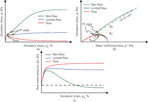
Undrained responses of sands in the (a) q–ϵq, (b) q–p′ and (c) Δu–ϵq spaces. PT, phase transmission; CSL, critical state line
Undrained responses of sands in the (a) q–ϵq, (b) q–p′ and (c) Δu–ϵq spaces. PT, phase transmission; CSL, critical state line
The CSSM framework is elegant and more widely evaluated with experimental data for granular materials after isotropic consolidation than K0 consolidation. However, there are experimental evidences that the consolidation history may affect the undrained response of sand and its corresponding CS behaviour. For instance, Finno and Rechenmacher (2003) reported that the location of CSL is affected by the consolidation history and initial state (i.e. before consolidation) of sand. The study of Fourie and Tshabalala (2005) found different CSLs for isotropically and K0-consolidated specimens. They also found that ηIS values of K0 consolidation were higher than those of isotropic consolidation. However, many other studies found a unique CSL for a soil regardless of consolidation condition (Kato et al., 2001). The uniqueness or non-uniqueness of CSL for different consolidations is a significant consideration for establishing the CSSM framework and its application for engineering practice. Due to the disagreement in literature, the effect of consolidation on the CS behaviour of soil requires further investigation.
Recognising the limitations of element tests under laboratory conditions, such as the sensitivity of monitoring transducers, disturbance/non-uniformity of specimens and shear band formation, the discrete-element method (DEM) has been gaining popularity for the qualitative understanding of soil behaviour under the CSSM framework. DEM does not have the same limitations as laboratory experimentation and also allows the understanding of particle interactions. There are published studies on CS behaviour of the assembly of two-dimensional circular and three-dimensional (3D) spherical particles (Huang et al., 2014; Kuhn, 2016; Sitharam and Vinod, 2009; Yan and Dong, 2011; Zhao and Guo, 2013); however, there is no detailed study on the effect of isotropic and K0 consolidations on undrained response, its characteristic features and CS behaviour.
Therefore, the objectives of this study are to (a) evaluate the effect of isotropic and K0 consolidations on undrained behaviour of saturated yellow silty (YS) sand and DEM simulations of 3D cubical assembly of ellipsoid particles under triaxial condition. This study did not attempt to simulate undrained behaviour of YS sand; rather, it attempted to evaluate undrained characteristic features – for example, ηIS, PT and CS – of granular materials that were observed for both laboratory triaxial test and DEM simulation. It is envisaged that such comparative evaluation between laboratory test and DEM will lead to the better understanding of the fabric-dependent behaviour of granular materials – for example, Yoshimine et al. (1998) and Li and Dafalias (2012); (b) evaluate unique/non-unique CSLs for isotropic and K0 consolidations; (c) evaluate the correlation for the undrained characteristic features – for example, PT state and ηIS – with state indices; and (d) evaluate the correlation for micromechanics measures such as particle contact and fabric anisotropy with state indices. This study enhances the understanding of the fundamental basis of the relationship between macro- or micromechanical responses and state indices of cohesionless granular materials.
Materials and methodologies
This study is composed of the triaxial testing of YS sand and the discrete element simulation of 3D ellipsoid particles. The physical properties of YS sand and the numerical properties of ellipsoid particles as well as laboratory testing and numerical simulation methodologies are explained below.
YS sand and 3D ellipsoid particles
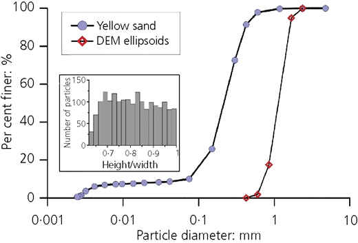
The YS sand, from South Australia, was used in this study. It is poorly graded and contained about 10% fines (poorly graded silty sand (SP-SM) according to the Unified Soil Classification System (USCS)), where fines are particles that have sizes smaller than 0·075 mm. The minimum and maximum void ratios are 0·423 (1·86 g/cm3) and 0·892 (1·40 g/cm3), respectively, according to ASTM D 4253 (ASTM, 2016) and ASTM D 698 (ASTM, 2017) methods, respectively. The clean sand is uniform and subrounded in nature. The fines were obtained by wet sieving of YS sand and classified as low plastic silt (ML) according to USCS which have a liquid limit (LL) and plasticity index (PI) of 40·0% and 9·3%, respectively.
The reason for using 3D elliptical particles is to capture an essence of angularity and reduce the computational demand as required for clustered particles. The grain size distribution curve of YS sand and 3D ellipsoids with their distribution of eccentricity – that is, height to width ratios – are shown in Figure 2. It is noted that the sizes and shapes of individual grains and specimens for laboratory testing and DEM simulation were different. Ellipsoid particles in DEM were larger and smoother than natural YS sand particles. A smaller and cubical specimen was used for DEM simulation, whereas a large cylindrical specimen was used in laboratory triaxial testing. These variations are commonly adopted for DEM simulations for simplicity and less computational demand as reported in many studies (Gu et al., 2014; Huang et al., 2014). As this study did not attempt to simulate YS sand behaviour with DEM, it rather attempted to evaluate the characteristic features that was reported for both laboratory triaxial test and DEM simulations, and the objective of this study was not significantly influenced by these variations. The DEM particles were assigned a normal contact stiffness of 108 N/m, ratio of tangential to normal contact stiffness of 1, coefficient of friction at particle contacts of 0·5 and the coefficient of (rotational and translational) body damping of 0·05.
Laboratory triaxial testing
Specimen preparation method
Different specimen preparation methods have been used in the literature such as air pluviation, water sedimentation and moist tamping for triaxial testing. Each method offers different advantages in resembling certain field conditions and fabrics. The moist tamping method provides two advantages for this study: (a) it produces very loose specimen suitable for liquefaction studies (Yamamuro and Lade, 1997) and (b) it reduces segregation of fines particles (Baki et al., 2012; Ladd, 1978; Rahman, 2009), which was a concern for YS sand. Therefore, a modified moist tamping method was adopted in this study (Bobei et al., 2009; Lo et al., 2010). A moist tamped specimen provides an initial soil fabric more representative of sandy deposits placed on land by end tipping, such as embankment fill or colluvium (Rahman et al., 2014a).
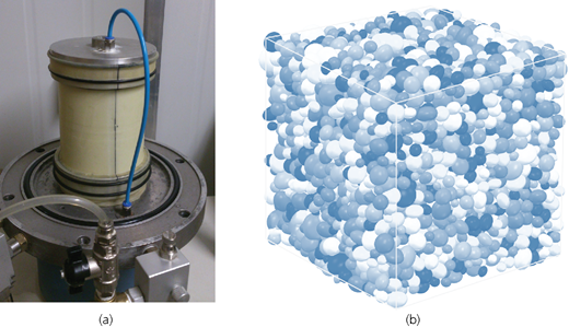
A 100 mm dia. and 100 mm high split mould of was placed over the enlarged bottom platen with free end, and a small vacuum of approximately −10 kPa was applied to hold the membrane inside this mould. The moist sand was tamped in ten layers to increase the homogeneity and reduce the variation in local density between neighbouring layers. The thickness of each layer was controlled using a height-controlled tamping rod. Free ends with enlarged platen reduce end restraint to a minimal value as verified in a number of studies on silt size to sand size materials (Bobei et al., 2009; Lo and Wardani, 2002; Lo et al., 2010). Figure 3(a) shows a specimen just after dismantling the split mould. Note that specimens with height-to-diameter ratio were unity, because it (a) was easier to prepare in terms of controlling uniformity of initial density and (b) minimised the likelihood and extent of specimen tilting during shearing. This approach has been well documented in literatures (Baki et al., 2014; Bobei et al., 2013; Chu et al., 1993; Rahman et al., 2008; Yamamuro and Lade, 1998; Zhang et al., 2018).
Saturation method
Carbon dioxide (CO2) was pumped into the specimen through the bottom platen for at least 10 min before the dismantlement of the split mould. Then saturation was performed in two stages: vacuum flushing and back pressure saturation. In stage 1, the specimen was flushed under the vacuum of −20 kPa overnight with de-aired water, and then in stage 2, a back pressure of 400 kPa was applied maintaining a p′ of 20 kPa. The specimen was left to rest with the back pressure for approximately 5 h to help dissolve any remaining air in the water. In most cases, a Skempton’s B value of 0·98 or higher was achieved in each test to ensure adequate saturation.
Isotropic consolidation module
The consolidation was conducted using a computer control module. During isotropic consolidation, the module increased cell pressure to the target cell pressure at specified intervals while allowing pore-water drainage to keep the pore-water pressure (back pressure) constant. While increasing isotropic cell pressure (σ1 = σ2 = σ3), the q was maintained constant to the user-defined value, usually q = 1 kPa, in the bedding control. Although the bedding control was not necessary for isotropic consolidation, it was maintained for consistency with other testing – for example, K0 consolidation and extension test. The digital pressure volume controller (DPVC) was used to measure the volume change during isotropic consolidation as well as keeping back pressure constant. Independent pressure transducers were used just outside the cell to check pore-water pressure equilibrium.
K0 consolidation module
First, a constant axial strain rate was applied, producing an increase in the effective vertical stress () up to the target value. For the applied vertical strain, zero radial strain was enforced by the DPVC in the manner described by Menzies (1988). In this module, a feedback system calculated the change of specimen volume (Δv) equal to the axial deformation increment multiplied by the current cross-sectional area of the specimen for a time step (default: 6 s). The time step was adjustable depending on the material response. The feedback system then commanded the DPVC to extract the volume of Δv to maintain zero radial strain – that is, ϵv = ϵ1 as shown in the following.
where ϵv is the volumetric strain. The extraction of volume causes a subsequent reduction to the pore pressure u (back pressure). To avoid the potential problem that a lower pore pressure may cause partial desaturation, the program commands the cell pressure regulator to increase the cell pressure by the drop in pore pressure. As change in pore pressure, Δu = BΔ3, where B is Skempton’s pore pressure parameter, and assuming that the specimen is nearly saturated (B ≈ 1), this action will restore the back pressure to the desired level. If B is somewhat less than 1, then there may be a lag in the restoration of the back pressure.
Once the consolidation is completed, the program has two exit modes, either ‘freeze stress’ or ‘freeze strain’. In the freeze stress mode, the control program keeps cell pressure, deviator stress and back pressure at their final values. Granting that pore pressures may still be equalising to some degree, and that the specimen may creep a small amount, the final K0 condition may be compromised if the specimen is held in this state for a protracted length of time. On the other hand, in the freeze strain mode, the ram is stopped at the exit of K0 consolidation – that is, axial strain is fixed, and the DPVC ceases volume change and reverts to pore pressure measurement. The cell pressure and pore pressure remain constant, but the deviator stress may keep changing slightly, depending on specimen stiffness. In this study, the freeze stress exit mode was used for all the tests.
Undrained shearing
The axial force was applied to the specimens at a constant deformation rate, and the cell pressure was kept constant at the initial value. In the undrained condition, the DPVC did not allow volume change, but the change of pore water pressure was measured.
DEM simulation of triaxial testing
The DEM software called Oval, developed by Kuhn (2006), was used for this study. The 3D ellipsoids assembly of cubical specimen under triaxial condition was simulated. Two methods were employed for preparing ellipsoid assemblies: staged isotropic consolidation and particle elimination (discussed later). A linear contact model and periodic boundary condition were considered in this study.
Staged isotropic consolidation
A staged isotropic consolidation approach, similar to that of Guo and Zhao (2013), was employed to achieve different densities. A set of specimens with a large number of particles (particle number N varied from 4350 to 5400) with the same grain size distribution was randomly generated in cubical 3D space. It is noted that there was no contact between particles at the beginning of this stage. The particles were then assigned with varying coefficients of friction at particle contacts (0–0·50) and 3D isotropic stress () up to 20 kPa was applied to achieve a desired void ratio. A higher coefficient of friction was used to generate a loose assembly. Note that after this stage, the coefficient of friction of all simulations was 0·50.
Particle elimination
The staged isotropic consolidation introduces different stress histories for different coefficients of friction at particle contacts during consolidation of up to 20 kPa. To avoid this, a new specimen preparation method was sought, and the particle elimination method was developed. In this method, a reference specimen was firstly achieved with ellipsoid with a very high density at p′ of 20 kPa by the staged isotropic consolidation. A MatLab code was developed to eliminate some ellipsoid particles from a dense specimen in such a way that the grain size distribution and particle orientation remained the same. This is discussed by Nguyen et al. (2017). An example of ellipsoid assembly is shown in Figure 3(b). The smaller specimen size for this study was approximately 9·33 × 9·33 × 9·33 mm3. The equivalence of undrained behaviour of specimens prepared by these two methods was observed and discussed by Nguyen et al. (2017).
Numerical challenges in DEM
A representative elementary volume (REV), which is the smallest volume that can yield a representative value of the whole, is important for numerical simulation. To achieve an REV condition in DEM simulations, micromechanical measures, such as inertial number (I), pseudostatic measures and specimen size, were examined in this study.
The quasi-static conditions of the DEM simulations were checked and maintained by analysing the inertial number (I), which is given by the following equation.
where is shear strain rate (1/s), d is the particle diameter (m), p′ is the mean stress (kPa), and ρg is the particle density (kg/m3). The particle density (ρg) was 9·766 × 108 kg/m3, which is approximately 3·69 × 105 times larger than 2650 kg/m3 for real geomaterial as reported by Perez et al. (2016). To optimise the simulation time, the particle density was scaled up in the literature, and notably, Thornton (2000) used a scale-up factor of 1012. A similar scale-up approach was also observed by Ng (2006). The strain rate of 0·00001% per time step was found as suitable for all DEM simulations (Nguyen and Rahman, 2017; Nguyen et al., 2015). The calculated I values for all simulations in this study were much smaller than the recommended value of 0·003 for quasi-static conditions (da Cruz et al., 2005).
Two variables, χ1 and χ2, were also checked to determine the numerical stability of the simulation. χ1 is the average force imbalance on a particle divided by the average magnitude of a contact force. χ2 is the average moment imbalance on a particle divided by both the average magnitude of a contact force and the average particle radius. For the applied strain rate, the highest values of χ1 and χ2 were below the recommended value of 0·005 (Kuhn, 2006) and considered that simulations were quasi-static.
Controlling module in DEM simulation
The Oval software allows a flexible stress or strain control triaxial simulation scheme by a six-digit input variable ‘icontr’, which represents the components of three principals in 11, 22 and 33 directions, and three shear 12, 13 and 23 directions. It should be noted that there are nine directions (i.e. three principal and six shear directions). However, the components in the directions 12 and 21, 13 and 31, 23 and 32 have the same magnitude but opposite direction. The different conditions in DEM simulations were achieved by adjusting these six components. The details are presented in the following.
Isotropic consolidation. The rates of change of principal stresses are the same – that is, . Note that single digit notations for principal stresses – that is, 1, 2 and 3 – were used in subscript when explaining the triaxial testing.
K0 consolidation. For an applied rate of major principal stress, the lateral strains are maintained constant or no lateral deformation – that is, dϵ22 = dϵ33 = 0.
Undrained shearing. For an applied axial strain rate, the volume of the assembly is maintained constant by adjusting the lateral strains. There was no pore water pressure development (Δu) during DEM simulation. However, it was determined by the difference between p′ for drained and undrained paths as explained by Sitharam et al. (2008) and Nguyen et al. (2018).
Micromechanical quantities
DEM allows the examination of particle interactions or contacts to establish links with the macroresponse of granular materials. Therefore, the coordination number (CN) and mechanical coordination number (Zm), as defined by Rothenburg and Bathurst (1989) and Thornton (2000), respectively, were used in this study. They can be mathematically expressed as follows.
where CN is the coordination number, C is the total number of contacts, N is the number of particles, N0 is the number of particles having no contact and N1 is the number of particles having only one contact in the specimen. Note that previous studies showed that Zm > CN, and their evolution paths are parallel during undrained shearing (Nguyen et al., 2017). Therefore, CN, instead of Zm, is used to synthesise the simulation data.
The structural anisotropy can be determined by the fabric tensor F, which was firstly introduced by Satake (1982) and expressed in the following equation.
where nk is the direction (unit vector) of the kth contact and N is the number of contacts in the specimen. The bold character (e.g. F) indicates the tensor, whereas the italic character (e.g. Fij) indicates the scalar value of the tensor. F11, F22 and F33 are the fabric in the principal directions (i = j), and F12, F13, F21, F23, F31 and F32 are the fabric in the shear directions (i ≠ j). As mentioned earlier, the scalar values of shear components in opposite direction are equal – that is, F12 = F21, F13 = F31 and F23 = F32. The fabric tensor can be formulated based on the theory of Cauchy stress tensor (σ), and the deviatoric fabric tensor (sF) can be expressed as
where
where the notation ‘tr(…)’ indicates the trace of a tensor and δij is Kronecker delta. sF has a set of invariants – for example, J1, J2 and J3 – and its characteristic equation can be written as
where λ is the constant of proportionality. The invariants of sF can be defined as
Based on von Mises stress yield criterion, a similar scalar quantity of equivalent deviatoric fabric – that is, von Mises fabric (FvM) – can be defined as
Comparison of isotropic and K0 consolidation: triaxial test and DEM simulation
Figure 4(a) shows four pairs of isotropic and K0 consolidation paths for the same preconsolidation e for both triaxial and DEM simulations in the e–log(p′) space. Although the loose triaxial test pair (YS-CIU05 and YS-K0U13) had approximately the same preconsolidation e of 0·670, the K0 consolidation path showed higher compression. Similarly, the dense triaxial test pair (YS-CIU15 and YS-K0U08) had approximately the same preconsolidation e of 0·590, the K0 consolidation path showed slightly higher compression. However, the difference of compressibility for isotropic and K0 consolidations was higher for higher preconsolidation e. Similarly, the loose (DE-CIU24 and DE-K0U04) and dense (DE-CIU21 and DE-K0U03) pairs from DEM simulations showed different compressibilities for different consolidation paths. The K0 consolidation paths showed slightly higher compression than isotropic consolidation, which increases with e. The purpose of Figure 4 is not to compare quantitatively the results from experiments and DEM simulations, but to capture the change in compressibility for isotropic and K0 consolidations and the trend of increasing compressibility with e for YS sand and other experimental studies (Butterfield and Marchi, 2017; Wong et al., 2017). Figure 4(b) shows the stress ratio () evolution paths of the triaxial tests and DEM simulations (presented in Figure 4(a)) in the space. It shows that K = 1 was maintained for isotropic consolidation; however, the K quickly dropped from 1 at the early stage of K0 consolidation (approximately ) and then gradually tends to reach a constant value at a higher stress level (approximately ). It seems that the constant K – that is, K0 value – is dependent on the preconsolidation e of DEM simulation. For instance, the preconsolidation e values of DE-K0U03 and DE-K0U04 were 0·540 and 0·634, respectively, and the loose specimen showed an early drop of K at lower than the dense specimen, but it achieved a higher K0 than the dense specimen – that is, K0 increases with e. Similarly, the loose triaxial specimen (YS-K0U13) showed an early drop of K at lower ; however, the test was terminated at a smaller (to maintain the same p′ of YS-CIU05) and could not confirm that K0 increases with e. However, in general, it was found for triaxial tests that the value of K0 increases with preconsolidation e. This observation differs from the widely used Jaky (1944) equation – that is, K0 = 1 – sin θm, which suggests that K0 only depends on the mobilised angle of internal friction (θm).
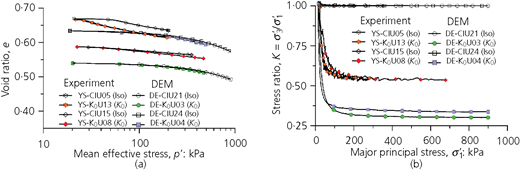
Isotropic and K0 consolidation paths in triaxial test and DEM simulation: (a) in e–log(p′) and (b) in space
Isotropic and K0 consolidation paths in triaxial test and DEM simulation: (a) in e–log(p′) and (b) in space
The micromechanical quantities – that is, CN and FvM from the DEM simulations – also depicted the difference in consolidation history as shown in Figure 5. Starting at the same value, the CN evolved to a much lower value under K0 condition than the CN under isotropic condition (Figure 5(a)). Note that higher CN implies stable state. Since K0 has lower CN, it shows higher compressibility in Figure 4(a) than isotropic consolidation. Figure 5(b) shows that FvM fluctuates around zero during isotropic condition. On the other hand, FvM quickly increases at a low for K0 condition and then reaches equilibrium at a higher . It is noted that micromechanical quantities – for example, CN and FvM – tend to reach equilibrium at a higher , which is very similar to macromechanical behaviour – that is, evolution in the space in Figure 4(b). In other words, the micromechanical measures seem to be able to reflect the macromechanical quantities.
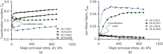
The evolution of micromechanical quantities during isotropic and K0 consolidations: (a) in space and (b) in space
The evolution of micromechanical quantities during isotropic and K0 consolidations: (a) in space and (b) in space
Results of triaxial tests and DEM simulations
A series of undrained triaxial compression tests for 21 isotropic and 14 K0 consolidated specimens was conducted. The range of e0 values was 0·497–0·655 and varied from 50 to 500 kPa, where subscript ‘0’ denotes the start of shearing. The details of these tests are presented in Table 1. Another series of DEM simulations under undrained triaxial condition for 54 isotropic and 15 K0 consolidated specimens was conducted (Table 2). The range of e0 values was 0·395–0·729 and varied from 19 to 1000 kPa. Some of these undrained simulations were part of another project and previously published by Nguyen et al. (2017).
The detail of triaxial tests
| Test number | e0 | : kPa | : kPa | OB | ψ0 | Dr |
|---|---|---|---|---|---|---|
| YS-CIU01 | 0·643 | 100 | 3 | F | 0·053 | 0·531 |
| YS-CIU02 | 0·655 | 200 | 6 | F | 0·085 | 0·504 |
| YS-CIU03 | 0·645 | 350 | 5 | F | 0·099 | 0·527 |
| YS-CIU04 | 0·642 | 100 | 5 | F | 0·052 | 0·533 |
| YS-CIU05 | 0·629 | 200 | 10 | F | 0·059 | 0·561 |
| YS-CIU06 | 0·610 | 300 | 5 | F | 0·056 | 0·601 |
| YS-CIU07 | 0·625 | 350 | 17 | F | 0·079 | 0·569 |
| YS-CIU08 | 0·628 | 50 | 3 | F | 0·025 | 0·563 |
| YS-CIU09 | 0·614 | 100 | 3 | F | 0·024 | 0·592 |
| YS-CIU10 | 0·607 | 200 | 13 | F | 0·037 | 0·608 |
| YS-CIU11 | 0·608 | 350 | 12 | F | 0·062 | 0·605 |
| YS-CIU12 | 0·600 | 100 | 19 | F | 0·010 | 0·622 |
| YS-CIU13 | 0·599 | 200 | 30 | F | 0·029 | 0·625 |
| YS-CIU14 | 0·595 | 200 | 30 | F | 0·025 | 0·633 |
| YS-CIU15 | 0·564 | 350 | 292 | F | 0·018 | 0·699 |
| YS-CIU16 | 0·539 | 200 | 283 | NF | −0·031 | 0·753 |
| YS-CIU17 | 0·527 | 350 | 589 | NF | −0·019 | 0·778 |
| YS-CIU18 | 0·493 | 100 | 575 | NF | −0·097 | 0·851 |
| YS-CIU19 | 0·480 | 350 | 771 | NF | −0·066 | 0·879 |
| YS-CIU20 | 0·621 | 100 | 3 | F | 0·031 | 0·578 |
| YS-CIU21 | 0·602 | 200 | 21 | F | 0·032 | 0·618 |
| YS-K0U01 | 0·531 | 170 | 97 | LF | −0·008 | 0·769 |
| YS-K0U02 | 0·514 | 260 | 202 | LF | −0·013 | 0·806 |
| YS-K0U03 | 0·516 | 364 | 148 | LF | 0·005 | 0·802 |
| YS-K0U04 | 0·515 | 492 | 368 | LF | 0·018 | 0·804 |
| YS-K0U05 | 0·562 | 108 | 8 | F | 0·017 | 0·704 |
| YS-K0U06 | 0·556 | 201 | 3 | F | 0·025 | 0·716 |
| YS-K0U07 | 0·555 | 278 | 31 | F | 0·034 | 0·719 |
| YS-K0U08 | 0·553 | 468 | 121 | LF | 0·054 | 0·723 |
| YS-K0U09 | 0·584 | 137 | 3 | F | 0·044 | 0·657 |
| YS-K0U10 | 0·573 | 211 | 6 | F | 0·043 | 0·680 |
| YS-K0U11 | 0·573 | 272 | 10 | F | 0·051 | 0·680 |
| YS-K0U12 | 0·559 | 371 | 19 | F | 0·049 | 0·710 |
| YS-K0U13 | 0·614 | 193 | 3 | F | 0·082 | 0·594 |
| YS-K0U14 | 0·479 | 243 | 624 | NF | −0·046 | 0·881 |
OB, observed behaviour; NF, non-flow; LF, limited flow; F, flow
The details of DEM simulations
| Simulation number | e0 | : kPa | : kPa | OB | ψ0 | DI0 | CN0 |
|---|---|---|---|---|---|---|---|
| DE-CIU01 | 0·538 | 50 | 1500 | NF | −0·130 | 0·606 | 7·738 |
| DE-CIU02 | 0·412 | 50 | 3268 | NF | −0·256 | 0·999 | 8·443 |
| DE-CIU04 | 0·582 | 50 | 809 | NF | −0·086 | 0·467 | 7·439 |
| DE-CIU05 | 0·631 | 50 | 393 | NF | −0·037 | 0·312 | 6·929 |
| DE-CIU07 | 0·660 | 100 | 3 | F | 0·000 | 0·193 | 5·283 |
| DE-CIU09 | 0·625 | 300 | 321 | NF | −0·011 | 0·223 | 5·760 |
| DE-CIU10 | 0·609 | 600 | 577 | LF | 0·003 | 0·174 | 6·230 |
| DE-CIU11 | 0·633 | 216 | 335 | NF | −0·012 | 0·228 | 5·401 |
| DE-CIU12 | 0·676 | 50 | 2 | F | 0·008 | 0·172 | 4·457 |
| DE-CIU13 | 0·678 | 50 | 1 | F | 0·010 | 0·165 | 4·305 |
| DE-CIU14 | 0·670 | 100 | 1 | F | 0·010 | 0·161 | 4·534 |
| DE-CIU15 | 0·729 | 19 | 0·231 | F | 0·055 | 0·033 | 4·437 |
| DE-CIU16 | 0·704 | 28 | 1 | F | 0·032 | 0·100 | 4·407 |
| DE-CIU17 | 0·687 | 36 | 1 | F | 0·016 | 0·148 | 4·370 |
| DE-CIU18 | 0·642 | 150 | 169 | NF | −0·012 | 0·228 | 5·136 |
| DE-CIU19 | 0·635 | 200 | 284 | NF | −0·012 | 0·228 | 5·373 |
| DE-CIU21 | 0·492 | 900 | 1981 | NF | −0·088 | 0·546 | 8·162 |
| DE-CIU24 | 0·573 | 900 | 936 | LF | −0·008 | 0·220 | 7·659 |
| DE-CIU26 | 0·659 | 100 | 3 | F | −0·001 | 0·195 | 4·746 |
| DE-CIU27 | 0·647 | 200 | 118 | LF | 0·001 | 0·187 | 5·346 |
| DE-CIU29 | 0·666 | 75 | 2 | F | 0·002 | 0·189 | 4·745 |
| DE-CIU30 | 0·577 | 1000 | 921 | LF | 0·005 | 0·172 | 6·596 |
| DE-CIU31 | 0·631 | 357 | 269 | LF | 0·002 | 0·179 | 5·831 |
| DE-CIU33 | 0·579 | 100 | 887 | NF | −0·081 | 0·454 | 7·518 |
| DE-CIU34 | 0·628 | 100 | 401 | NF | −0·032 | 0·297 | 7·164 |
| DE-CIU35 | 0·648 | 100 | 251 | NF | −0·012 | 0·232 | 6·567 |
| DE-CIU36 | 0·639 | 200 | 235 | NF | −0·007 | 0·213 | 6·900 |
| DE-CIU37 | 0·632 | 285 | 371 | NF | −0·005 | 0·202 | 6·956 |
| DE-CIU38 | 0·629 | 335 | 348 | NF | −0·003 | 0·197 | 6·964 |
| DE-CIU39 | 0·631 | 240 | 315 | NF | −0·011 | 0·225 | 5·617 |
| DE-CIU40 | 0·632 | 230 | 282 | NF | −0·011 | 0·226 | 5·579 |
| DE-CIU43 | 0·496 | 50 | 1964 | NF | −0·172 | 0·736 | 7·966 |
| DE-CIU44 | 0·455 | 50 | 2521 | NF | −0·213 | 0·865 | 8·178 |
| DE-CIU48 | 0·615 | 600 | 498 | LF | 0·009 | 0·153 | 5·870 |
| DE-CIU61 | 0·514 | 480 | 1550 | NF | −0·103 | 0·560 | 7·960 |
| DE-CIU62 | 0·599 | 498 | 691 | NF | −0·016 | 0·244 | 7·494 |
| DE-CIU63 | 0·625 | 300 | 338 | NF | −0·011 | 0·223 | 5·743 |
| DE-CIU64 | 0·625 | 300 | 350 | NF | −0·011 | 0·223 | 5·743 |
| DE-CIU65 | 0·497 | 100 | 1959 | NF | −0·163 | 0·718 | 7·307 |
| DE-CIU66 | 0·470 | 600 | 2389 | NF | −0·136 | 0·696 | 7·661 |
| DE-CIU67 | 0·450 | 1000 | 2616 | NF | −0·123 | 0·698 | 7·843 |
| DE-CIU51 | 0·611 | 600 | 590 | NF | 0·005 | 0·166 | 5·327 |
| DE-CIU52 | 0·660 | 107 | 4 | F | 0·001 | 0·190 | 4·517 |
| DE-CIU53 | 0·667 | 100 | 3 | F | 0·007 | 0·171 | 4·289 |
| DE-CIU54 | 0·673 | 100 | 2 | F | 0·013 | 0·151 | 4·325 |
| DE-CIU55 | 0·679 | 100 | 0·224 | F | 0·019 | 0·132 | 4·184 |
| DE-CIU56 | 0·661 | 50 | 4 | F | 0·000 | 0·220 | 4·161 |
| DE-CIU57 | 0·613 | 600 | 581 | LF | 0·007 | 0·158 | 5·541 |
| DE-CIU58 | 0·558 | 600 | 1213 | NF | −0·048 | 0·366 | 6·046 |
| DE-CIU59 | 0·580 | 600 | 1014 | NF | −0·026 | 0·285 | 5·604 |
| DE-CIU60 | 0·620 | 600 | 498 | LF | 0·014 | 0·133 | 5·509 |
| DE-CIU68 | 0·497 | 100 | 1939 | NF | −0·163 | 0·718 | 7·135 |
| DE-CIU69 | 0·470 | 600 | 2382 | NF | −0·136 | 0·696 | 7·471 |
| DE-CIU70 | 0·450 | 1000 | 2660 | NF | −0·123 | 0·698 | 7·657 |
| DE-K0U02 | 0·395 | 459 | 3800 | NF | −0·224 | 0·996 | 8·087 |
| DE-K0U03 | 0·511 | 481 | 1548 | NF | −0·106 | 0·571 | 7·121 |
| DE-K0U04 | 0·592 | 502 | 736 | NF | −0·023 | 0·269 | 6·379 |
| DE-K0U05 | 0·684 | 68 | 1 | F | 0·019 | 0·135 | 4·120 |
| DE-K0U06 | 0·694 | 36 | 0·384 | F | 0·023 | 0·127 | 4·106 |
| DE-K0U08 | 0·661 | 94 | 2 | F | 0·000 | 0·194 | 4·744 |
| DE-K0U11 | 0·668 | 68 | 1 | F | 0·004 | 0·184 | 4·336 |
| DE-K0U14 | 0·673 | 52 | 1 | F | 0·006 | 0·179 | 4·173 |
| DE-K0U15 | 0·616 | 562 | 579 | LF | 0·006 | 0·162 | 5·199 |
| DE-K0U17 | 0·607 | 514 | 582 | LF | −0·007 | 0·212 | 6·132 |
| DE-K0U18 | 0·551 | 492 | 1327 | NF | −0·065 | 0·423 | 6·888 |
| DE-K0U19 | 0·614 | 525 | 505 | LF | 0·001 | 0·182 | 5·699 |
| DE-K0U20 | 0·552 | 481 | 1246 | NF | −0·066 | 0·424 | 6·891 |
| DE-K0U23 | 0·698 | 29 | 0·472 | F | 0·040 | 0·120 | 4·153 |
| DE-K0U24 | 0·709 | 22 | 0·303 | F | 0·051 | 0·092 | 4·283 |
Undrained behaviour and characteristic feature
The F behaviours in q–p′ and q–ϵ q spaces after isotropic and K 0 consolidations of loose triaxial specimen and DEM simulation under triaxial conditions are presented in Figures 6(a) and 6(b) and Figures 6(c) and 6(d), respectively. The ESPs of two isotropic triaxial specimens (YS-CIU04 and YS-CIU05) started from q = 0 and raised to a peak q (q peak). The strain softening or static liquefaction – that is, dq/dϵ q < 0 – was triggered just after q peak. The η IS of YS-CIU04 and YS-CIU05 were 0·742 and 0·762, respectively, as shown by dotted lines in Figure 6(a). However, after K 0 consolidation, YS-K0U10 and YS-K0U11 reached the initial q of 135 and 193 kPa, respectively. During undrained shearing, the q of these two triaxial tests quickly rose to a q peak, and then strain softened to static liquefaction. The η IS of YS-K0U10 and YS-K0U11 were 0·726 and 0·796, respectively. There was no obvious correlation between η IS and consolidation type for these tests. This may be due to the fact that these tests had very different initial q, e and p′. The effect of these variables is discussed later. The stress–strain behaviour of these triaxial tests are shown in the q–ϵ q space in Figure 6(b). Interestingly, q peak occurred quickly for K 0-consolidated specimens (approximately 0·5% strain), whereas the q peak of isotropic consolidated specimen occurs at around 2–5% strain, as shown in Figure 6(b).
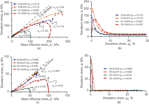
Undrained behaviours (F) of loose YS sand and DEM ellipsoids after isotropic and K 0 consolidations: (a) in q–p′ space (triaxial tests); (b) in q–ϵ q space (triaxial tests); (c) in q–p′ space (DEM); and (d) in q–ϵ q space (DEM)
Undrained behaviours (F) of loose YS sand and DEM ellipsoids after isotropic and K 0 consolidations: (a) in q–p′ space (triaxial tests); (b) in q–ϵ q space (triaxial tests); (c) in q–p′ space (DEM); and (d) in q–ϵ q space (DEM)
Similar to triaxial tests, the DEM simulation of loose assembly under triaxial condition showed q peak for both isotropic and K 0 consolidations as presented in Figure 6(c). However, η IS of DE-K0U05 and DE-K0U11 were 0·805 and 0·849, respectively, which were higher than η IS of 0·240 and 0·418 for DE-CIU13 and DE-CIU14, respectively. Note that η IS values for K 0 consolidated were significantly higher that isotropic consolidation. η, after K 0 consolidated corresponding to initial q at the start of undrained shearing, was somewhat close to the CS stress ratio M. The stress–strain behaviour of these DEM simulations showed a quick drop from q peak to q = 0 at CS as shown in Figure 6(d).
The NF behaviour in q–p′ and q–ϵ q spaces after isotropic and K 0 consolidations of dense triaxial specimen and DEM simulation under triaxial conditions are presented in Figures 7(a) and 7(b) and Figures 7(c) and 7(d), respectively. Usually, LF and NF responses exhibit the PT state at the knee of the ESP, which can be defined as the state of dp′ = 0 on the ESP in the q–p′ space (Lade and Ibsen, 1997). However, other researchers argued that the PT state separates the contractive to dilative tendency at dϵ v = 0; therefore, the equivalence of this for the undrained test would be dΔu = 0. Hence, Sukumaran et al. (1996) define PT state as a state of dΔu = 0. Although the triaxial test and DEM simulations in Figure 7 did not show the clear knee of ESP, the latter definition allowed the identification of PT states at dΔu = 0. The stress ratio at PT (η PT) on the ESP is considered as an important characteristic feature and has been used in constitutive formulation (Manzari and Dafalias, 1997; Wood et al., 1994). η PT in triaxial tests occurred below the M-line, and after that, ESPs follow the M-line as shown in Figure 7(a). It appears that both K 0 and isotropic consolidation tests tend to a unique CSL in the q–p′ space – that is, the M-line. Figure 7(c) shows that ESPs of DEM simulations evolved beyond the CSL (M-line) and then come back to CS at large strain (ϵ q > 15%). η PT was also higher than M. The stress–strain paths for both triaxial and DEM simulations showed very similar patterns of strain hardening as shown in Figures 7(b) and 7(d). Note that the Δu development in Figures 6 and 7 exhibits a similar pattern to what was observed in Figure 1(c), and Δu data for these tests are shown in Figures 1 and 2 in the online supplementary material.
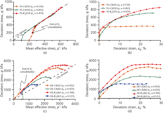
Undrained behaviour (NF) of dense YS sand and DEM ellipsoids after isotropic and K 0 consolidations: (a) in the q–p′ space (triaxial tests); (b) in the q–ϵ q space (triaxial tests); (c) in the q–p′ space (DEM); and (d) in the q–ϵ q space (DEM)
Undrained behaviour (NF) of dense YS sand and DEM ellipsoids after isotropic and K 0 consolidations: (a) in the q–p′ space (triaxial tests); (b) in the q–ϵ q space (triaxial tests); (c) in the q–p′ space (DEM); and (d) in the q–ϵ q space (DEM)
Relationship between density index and characteristic features
To evaluate the effect of density index, the relative density (D r) as defined in the following equation, was primarily used for triaxial specimen of YS sand.
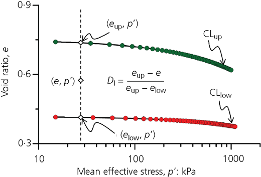
where e max and e min are the maximum and minimum void ratios, respectively. However, the measurements of e max and e min are challenging and problematic in DEM; therefore, an alternative measure of D r, called densification index (D I), was adopted to capture the density of the assembly of ellipsoids. D I was defined as the state of soil relative to the upper and lower boundary consolidation lines (see Figure 8) as proposed by Zhang et al. (2018). D I can be expressed as follows.
where e up and e low are the corresponding void ratios on upper and lower consolidation lines, respectively. The upper consolidation line (CLup) was the consolidation line of loosest assembly, whereas the consolidation line of densest assembly was the lower consolidation line (CLlow). So, the density indices for the triaxial tests and DEM simulation were D r and D I, respectively, in this study. Note that D r and D I are slightly different as D I is dependent on , and therefore, its value for the same e can change with consolidation pressure p′. However, if the isotropic consolidation lines (ICLs) are parallel, the value of D I does not change with p′.
Relationship between density index and ηIS state
The relationships between ηIS and the density indices – that is, Dr and DI – are shown in Figure 9 for both triaxial and DEM simulations. In general, ηIS was increased with Dr for both K0- and isotropically consolidated specimen in triaxial tests as shown in Figure 9(a). The root mean square deviation (RMSD) of the best-fit trend was 0·100. The Dr values of K0 tests were comparatively higher than that of isotropic tests, as e after K0 consolidation were mostly lower than e after isotropic consolidation (as shown in Figure 4(a)). Similarly, ηIS was increased with DI0 in the ηIS–DI0 space for both K0 and isotropically consolidated specimen in DEM simulation as shown in Figure 9(b), where DI0 is the densification index at the start of shearing. The RMSD of the best-fit trend was 0·268. The ηIS of K0 simulations seem to be higher than that of isotropic simulation. The CN at instability (CNIS) increased with DI0, but it did not exhibit any dependency on the consolidation type (the RMSD of this relation was 0·416) as shown in Figure 9(c). The FvM at instability (FvM,IS) also increased with DI0, and FvM,IS of K0 simulation seems to be higher than that of the isotropic simulation (the RMSD of this relation was 0·021) as shown in Figure 9(d). The pattern of the FvM,IS–DI0 relation in Figure 9(d) is somewhat similar to the ηIS–DI0 relation in Figure 9(b).
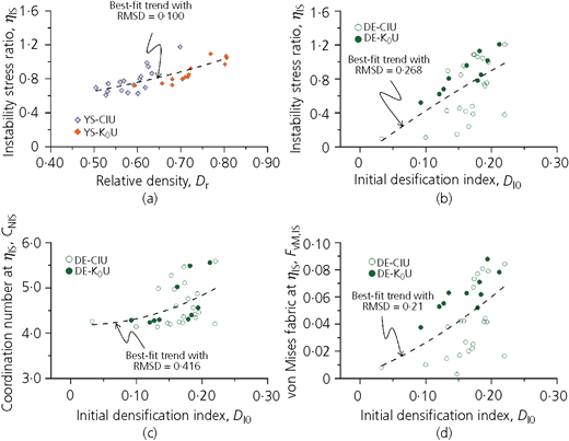
Relationship between instability state and density state: (a) in the ηIS–Dr space (triaxial test); (b) in the ηIS–DI0 space (DEM); (c) in the CNIS–DI0 space (DEM); and (d) in the FvM–DI0 space (DEM)
Relationship between instability state and density state: (a) in the ηIS–Dr space (triaxial test); (b) in the ηIS–DI0 space (DEM); (c) in the CNIS–DI0 space (DEM); and (d) in the FvM–DI0 space (DEM)
Relationship between density index and PT state
Figure 10(a) shows that the ηPT decreases with Dr in the ηPT–Dr space for triaxial tests. The best-fit trend for ηPT and Dr was higher for K0 consolidation than that of for isotropic consolidation. These two trends appear to meet at Dr = 0·90. However, the ηPT increased gradually with DI0 in the ηPT–DI0 space for DEM simulation as shown in Figure 10(b). Interestingly, the best-fit trend did not have any obvious dependency on consolidation type for the DEM simulations of this study, which is different from what was observed for triaxial data in Figure 10(a).
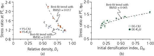
Correlations of ηPT: (a) with Dr in the ηPT–Dr space and (b) with DI0 in the ηPT–DI0 space
Correlations of ηPT: (a) with Dr in the ηPT–Dr space and (b) with DI0 in the ηPT–DI0 space
Relationship between density index and flow potential (uF)
The flow potential (uF), as defined in Equation 12, is often used to characterise granular material behaviour.
where is the mean effective confining stress at the PT state. Figure 11(a) shows that the uF decreases with Dr in the uF–Dr space for triaxial tests. The best-fit line has an RMSD of 0·361. Note that the uF values can be negative for higher than in Equation 12 – that is, the PT occurs at a higher stress level (p′) than the initial state of . Unlike the ηPT–DI0 relation in Figure 10(b), uF was decreased with DI0 in the uF–DI0 space, and two distinct relations were observed for isotropic and K0 consolidations for DEM simulation (see Figure 11(b)). Noticeably, most uF values of K0 simulations are relatively small, and some tend to negative.
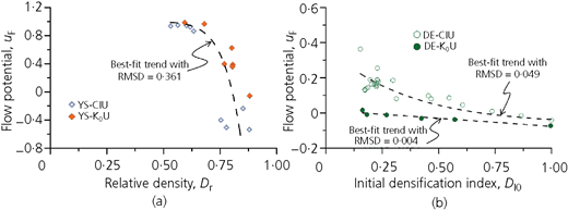
Correlations of uF: (a) with Dr in the uF–Dr space (triaxial tests) and (b) with DI0 in the uF–DI0 space (DEM)
Correlations of uF: (a) with Dr in the uF–Dr space (triaxial tests) and (b) with DI0 in the uF–DI0 space (DEM)
The above investigation suggests that the overall qualitative behaviour of YS sand in triaxial testing can be captured by DEM simulation for triaxial testing with a simple linear contact model for ellipsoid particles. However, there are disagreements between the experiment and DEM data for some characteristic features, which require further investigation and development. Since Dr and DI were not equivalent density indices, this study investigated the correlation of these characteristic features within the CSSM framework.
CSSM framework
This study revisited the classical CSSM framework and investigated the CS behaviour of the YS sands and DEM ellipsoids.
CS and CSL
Figure 12(a) shows a pair of ESPs for DEM simulations with almost the same e 0 of 0·592–0·599 and of 500 kPa after K 0 and isotropic consolidations. As previously shown in Figure 7(c), the ESPs for DE-CIU71 and DE-K0U04 evolved beyond the CSL (M-line) and then both the ESPs came back/approached towards the same CS (η = M) at the end of simulation (see Figure 12(a)). Note that the stress state of DE-K0U04 after K 0 consolidation or at the start of undrained shearing was higher than M as indicated by an arrow in Figure 12(a). The F vM paths for these simulations evolved to a narrow zone (see Figure 12(b)). This zone was termed as ‘CS zone’, which was in line with the concept of CS fabric as discussed by Dafalias (2016). Interestingly, both the ESP and F vM evolution paths were similar – that is, they go beyond the CS and come back to CS or a narrow zone – which suggests that F vM may be a good micromechanical parameter for characterising the macromechanical behaviour.
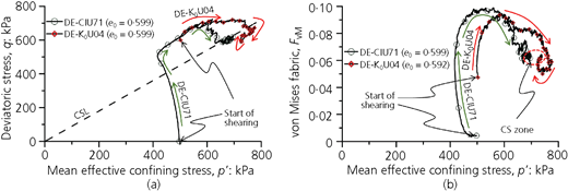
The evolution towards CS from DEM simulations in the (a) q–p′ space and (b) F vM–p′ space
The evolution towards CS from DEM simulations in the (a) q–p′ space and (b) F vM–p′ space
Most triaxial tests and DEM simulations in this study reached clear CS. However, in few cases in which a clear CS was not reached, an extrapolation method, as discussed by Rahman and Lo (2014), was used. In this method, the rate of change of excess pore pressure (dΔu/dϵ q) is plotted against η as shown in Figure 13 for both experimental and DEM data. The value of η at CS (M) can be estimated by extrapolating dΔu/dϵ q to 0. Then, p′ at the CS is estimated by extrapolating η to M in an η–p′ plot. Such an extrapolation approach was also employed in other studies presented in the literature (Carrera et al., 2011; Murthy et al., 2007; Zhang et al., 2018). In the case of dense specimen in DEM simulation, dΔu/dϵ q = 0 was achieved twice: at the PT state and at the CS as shown in Figure 13(b). However, for the loose specimen in triaxial test, dΔu/dϵ q becomes 0 at the CS (Figure 13(a)) – that is, PT and CS may coincide.
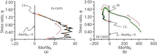
The extrapolation method for CS: (a) loose specimen (YS-CIU15, triaxial test) and (b) dense specimen (DE-CIU02, DEM)
The extrapolation method for CS: (a) loose specimen (YS-CIU15, triaxial test) and (b) dense specimen (DE-CIU02, DEM)
The CS data points from triaxial experiments formed two different CSLs in the e–log(p′) space for K 0 and isotropically consolidated specimens (Figure 14(a)). The finding of non-unique CSLs for YS sand for different consolidation conditions was somewhat unexpected and undesirable for the CS framework. This finding did not coincide with the authors’ earlier findings of unique CSL under triaxial compression, irrespective of drainage conditions, for Sydney sand (Rahman et al., 2014a), pond ash (Zhang et al., 2018) and Hostun sand (Goudarzy et al., 2017). Therefore, it has also been verified for different drainage conditions and confirmed. The details of these verifications are published in a separate article (Rabbi et al., 2018). Note that the non-unique CSLs for different consolidations is not new. Finno and Rechenmacher (2003) observed non-unique CSLs for undrained loading after anisotropic consolidations. Fourie and Tshabalala (2005) observed slightly different CSLs for undrained loading after isotropic and anisotropic consolidations (see Figure 15). However, the CS data points from DEM simulations of this study formed single CSL regardless of consolidation condition. Other DEM studies – for example, that of Zhou et al. (2017) – observed different critical state stress ratios (q/p′) for the drained condition after isotropic and anisotropic consolidations. However, they have not reported CSL in the e–log(p′) space. This suggested that the assumption of a presumptive unique CSL from triaxial experiment or DEM simulation is not necessarily true for all granular materials. Further research is required to understand the material properties that might lead to such deviation from unique CSL.
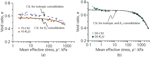
CSLs for isotropic and K 0 consolidation tests in the e–log(p′) space: (a) triaxial test and (b) DEM
CSLs for isotropic and K 0 consolidation tests in the e–log(p′) space: (a) triaxial test and (b) DEM
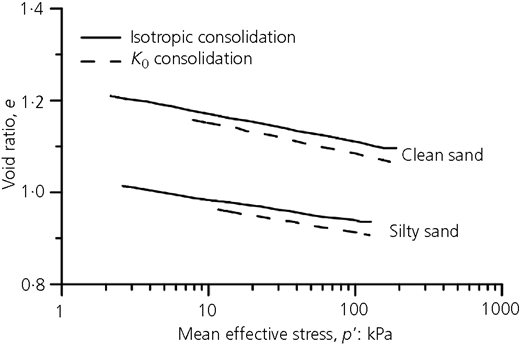
CSLs for triaxial tests after isotropic and K 0 consolidations, modified after Fourie and Tshabalala (2005)
CSLs for triaxial tests after isotropic and K 0 consolidations, modified after Fourie and Tshabalala (2005)
Figure 16(a) shows that the C N at CS forms unique relationships with p′. Figure 16(b) shows that F vM at CS in the F vM–p′ space also forms a unique narrow CS zone for both K 0 and isotropic simulations. Although it was previously reported that the fabric evolved during undrained shearing (see Figure 12(b)), Figure 16(b) suggested that all F vM values at CS formed a unique trend with the corresponding p′. Hence, the fabric anisotropy, which represents the internal structure of the specimen, evolved from an initial value towards a CS value. This supported the fabric evolution and CS fabric concept of the anisotropic critical state theory (ACST) by Li and Dafalias (2012), and Dafalias (2016). The evolution of F vM in this study was in fact a presentation of the fabric evolution in ACST. Although a fabric evolution model is already suggested for ACST, this study presents evidence for the evolution of fabric (see Figures 12(a) and 12(b)) and its relation with characteristic features to adopt necessary corrections on such model.
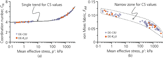
CS data for the micromechanical quantities – that is, (a) C N and (b) F vM in relation with p′ at CS
CS data for the micromechanical quantities – that is, (a) C N and (b) F vM in relation with p′ at CS
Relation between state parameter (ψ) and characteristic features
The CSL in the e–log(p′) space has been used as the reference state for soil behaviour. For example, a soil state above the CSL exhibits F behaviour, whereas a soil state below the CSL exhibits NF behaviour. A soil state with respect to CSL can be presented by a state index. One of the widely used state indices is the state parameter (ψ). Been and Jefferies (1985) defined ψ as the difference between the current e and the corresponding e on CSL at the same p′. A positive ψ – that is, e above CSL – exhibits F behaviour, whereas a negative ψ – that is, e below CSL – exhibits NF behaviour. The relation between the state parameter (ψ) and characteristic features on undrained behaviour are explored in the following subsection.
Relationship between state parameter (ψ) and ηIS
The ηIS and ψ0 data points for triaxial testing after K0 and isotropic consolidations showed a good relation, where ηIS decreased with increasing ψ0 (see Figure 17(a)). The overall trend is consistent with earlier studies for isotropic consolidated sands (Baki et al., 2012; Imam et al., 2002; Rahman and Lo, 2012; Rahman et al., 2014b; Yang, 2002). The best-fit line in this study has an RMSD of 0·100. However, one may notice that the ηIS data points for K0 consolidation were slightly higher than those for isotropic consolidation for higher ψ0. This behaviour was clearly observed for the ηIS–ψ0 relation in DEM simulation – that is, ηIS for K0 consolidation was significantly higher than that for isotropic consolidation for higher ψ0 (RMSDs for the relations after isotropic and K0 consolidations are 0·313 and 0·084, respectively), as shown in Figure 17(b). The unique relationship between CN at ηIS and ψ0 with RMSD of 0·364 is presented in Figure 17(c), which suggests that the difference between ηIS–ψ0 relations for K0 and isotropic consolidations are not dependent on CN. The FvM and ψ0 data points are presented in Figure 17(d), which shows that FvM–ψ0 for K0 consolidation was significantly higher than that for isotropic consolidation for higher ψ0 (RMSDs for the relations after isotropic and K0 consolidations are 0·021 and 0·010, respectively). This is similar to macromechanical behaviour – that is, the ηIS–ψ0 relation in Figure 17(b). This again suggests that the fabric quantity (FvM) may represent the macromechanical behaviour better than the number of contacts (CN).
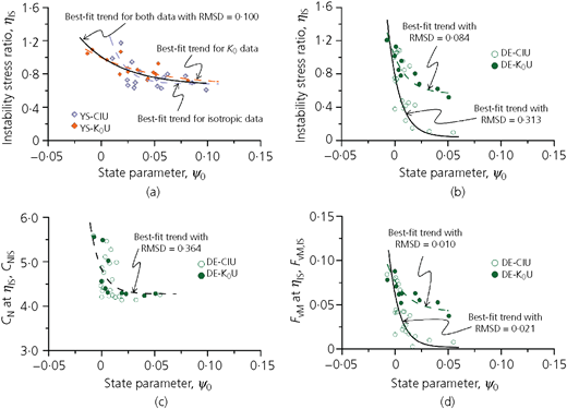
Relationship for ηIS and micromechanical quantities (CN and FvM) at ηIS with ψ0 for isotropic and K0 consolidations (a) in the ηIS–ψ0 space (triaxial tests), (b) ηIS–ψ0 space (DEM), (c) in the CIS–ψ0 space (DEM) and (d) in the FvM–ψ0 space (DEM)
Relationship for ηIS and micromechanical quantities (CN and FvM) at ηIS with ψ0 for isotropic and K0 consolidations (a) in the ηIS–ψ0 space (triaxial tests), (b) ηIS–ψ0 space (DEM), (c) in the CIS–ψ0 space (DEM) and (d) in the FvM–ψ0 space (DEM)
Relationship between state parameter (ψ) and ηPT
Figure 18(a) shows that η at the PT state (ηPT) form a unique relationship with ψ0 in the ηPT–ψ0 space for both isotropic and K0 triaxial experiments. The best-fit trend has an RMSD of 0·117. One may recall that these data exhibited separate trends in the ηPT–Dr space in Figure 10(a) for isotropic and K0-consolidated specimens. It appeared that ψ0, which captures the effect of e and p′, is a better state index than Dr. Figure 18(b) also shows the unique relationship between ηPT and ψ0 for both DEM isotropic and K0 simulations. The best-fit trend has an RMSD of 0·081. However, one may note that ηPT increased with ψ0 for triaxial data, whereas ηPT decreased with ψ0 for DEM data. While these are observed behaviours from this study, authors were cautious to draw a general conclusion that triaxial data are more reliable/acceptable than DEM. This is because (a) both triaxial and DEM simulations did not show a clear knee on the ESP at dp′ = 0, and an alternative approach of dΔu = 0 was used to identify the PT state; (b) Zhang et al.’s (2018) triaxial data also show a similar trend as observed for DEM simulation. Although the authors suggest further study on the shape of ηPT–ψ0 curve, ψ appeared as a better state of soil.
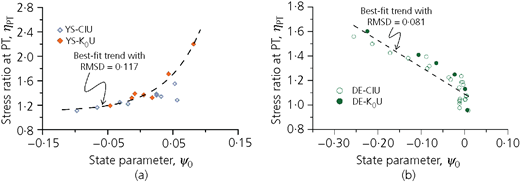
Relationship between ηPT and ψ0 for both (a) experiments and (b) DEM simulations
Relationship between ηPT and ψ0 for both (a) experiments and (b) DEM simulations
Relationship between state parameter (ψ) and uF
The uF–ψ0 relations for triaxial tests after isotropic and K0 consolidations are presented in Figure 19(a), which shows that uF increased with ψ0. These data were not dependent on consolidation type. The best-fit line for these data has an RMSDs of 0·280. The uF–ψ0 relations for DEM simulations of isotropic and K0 consolidations are presented in Figure 19(b). Unlike for the triaxial tests, these data showed two distinct relations for isotropic and K0 consolidations. The best-fit trend of the uF–ψ0 relation for isotropic consolidation has an RMSD of 0·046 and the best-fit line for K0 consolidation has an RMSD of 0·004.
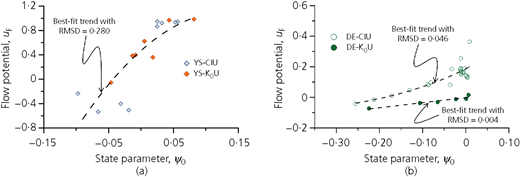
Relationship between uF and ψ0 for both (a) experiments and (b) DEM simulations
Relationship between uF and ψ0 for both (a) experiments and (b) DEM simulations
Conclusions
This study combined triaxial tests on YS sand and 3D DEM cubical assembly consisting of ellipsoids under triaxial condition to investigate the effect of consolidation condition on the overall undrained behaviour and its characteristic features. Both density indices and the CSSM framework were used to develop the correlations for characteristic features of undrained behaviour (often referred to as macromechanical behaviour). The micromechanical measures such as coordination number (CN) and fabric anisotropy (FvM) were evaluated to understand how the micromechanical behaviour affect the macromechanical behaviour. The major findings from this study are listed in the following.
For the same preconsolidation void ratio (e), the consolidation paths have a significant influence on the compressibility and post-consolidation void ratio (e0) for both triaxial and DEM simulations. The K0 consolidation path achieved higher compression than that of corresponding isotropic consolidation path. The DEM simulation showed that for isotropic loading – that is, – the CN increased with to achieve a stable state and exhibited lower compressibility, whereas CN initially decreased with for K0 consolidation, which may have contributed to higher compressibility. Similarly, the fabric anisotropy (FvM) evolved significantly during K0 consolidation, whereas FvM reduced during isotropic consolidation.
For loose specimen, the instability or static liquefaction was triggered just after peak deviatoric stress (qpeak) at instability stress ratio (ηIS). The K0-consolidated triaxial test reached the triggering of static liquefaction – that is, ηIS at a much smaller deviatoric strain (ϵq = 0·5%) than the deviatoric strain isotropic consolidated tests (ϵq = 2–3%). A similar behaviour was observed for the ESP in the DEM simulation. However, there was no conclusive evidence from the DEM simulation that static liquefaction would trigger at a much smaller ϵq for K0 consolidation than isotropic consolidation.
For a dense specimen, the ESP for both triaxial and DEM simulations after K0 and isotropic consolidations reached critical state stress ratio (M). However, the ESP for DEM simulation rose above the M-line and then turned back to M towards the end of the simulation. This behaviour is not very common for experimental studies.
The ηIS for loose specimen increases with relative density (Dr) for triaxial tests. Similarly, ηIS increased with density index (DI) for DEM simulation. The trend was not dependent on K0 or isotropic consolidation for both triaxial and DEM simulations. The micromechanical measures – for example, CN and FvM at instability – also increased with DI. Similarly, the characteristic features of the PT state also showed correlations with Dr and DI for triaxial and DEM simulations, respectively.
The critical state lines (CSLs) for YS sand were different in the e–log(p′) space for isotropic and K0 consolidations, where the CSL of K0 data was higher than that of isotropic data. However, the CSL for DEM simulation for isotropic and K0 consolidations was unique in the e–log(p′) space. The micromechanical measures – for example, CN and FvM at CS – also showed a unique relation with p′.
The ηIS for loose specimen decreased with ψ0 for both experiments and DEM simulations. However, the ηIS–ψ0 relation was different for isotropic and K0 consolidation types. The unique relation was observed between CNIS and ψ0 irrespective of consolidation type. The FvM–ψ0 relation was dependent on the consolidation type as observed for the ηIS–ψ0 relation. This suggests that the difference in the ηIS–ψ0 relation for different consolidation was not due to the change of CNIS but for FvM.
The ηIS and uF showed good correlation with density indices (Dr and DI) and ψ0.
This study was based on the experimental data for YS sand and DEM simulations of the 3D cubical assembly of ellipsoid particles with linear contact model. There were assumptions made on estimating PT states, extrapolation for CS and others. Therefore, reader should be cautious in generalising the outcome of this article.



Acknowledgements
The authors would like acknowledge Professor Matthew R. Kuhn of University of Portland, USA, for his discrete-element method software Oval. The second and third author would like to acknowledge the financial support of the University Presidents Scholarship and the University of South Australia Postgraduate Research Award from University of South Australia.

