


A new combined method for the inverse modelling of leakage from the body and foundation of earth dams considering a transient flow model is introduced in this paper. Reaching a unique result, an objective function that simultaneously employs the time series of hydraulic heads and observations of flow rates has been defined. An inclusive finite-element model that considers all the construction stages of an earth dam has been created and then orthogonal design, back-propagation artificial neural networks and a genetic algorithm have been used to do inverse modelling. The proposed method has been employed for the inverse modelling of leakage in Baft dam in Kerman, Iran. Hydraulic conductivities of different parts of the dam have been investigated for two distinct predefined cases, and in both cases satisfactory results have been obtained. The fitting results show the applicability of the suggested method in inverse modelling of real large-scale problems, which not only decreases the computation cost but also increases reliability and efficiency in such problems.
Notation
- K
vector of permeability values in various flow elements to be determined
different permeability states in orthogonal design
- Klow
lower bound of the possible permeability values
- Kup
upper bound of the possible permeability values
- ki
permeability value of the element i in K
- m
number of permeability values in the various flow elements
- m
number of piezometers installed on the whole domain
- n
number of flowmeters installed on the whole domain
- Q j(K)
time series of flow rates at flowmeter j resulting from an assumptive vector K
time series of flow rate readings in the flowmeter j
flow rate in the flowmeter j at time t
- w
weight parameter
- φ i(K)
time series of hydraulic heads at piezometer i resulting from an assumptive vector K
time series of hydraulic head readings in piezometer i
hydraulic head in piezometer i at time t
- Ω
domain
- ‖·‖2
Euclidean norm of a vector
Introduction
The permeability of deposits below a dam or in its body is one of the most important factors in the design of earth dams and affects the dam location and design of its water-sealing system. The main factors affecting the rate of permeability in rocks and soils are the geometric shape and the relationship between existing voids and cavities. Its value can be determined locally using field experiments. Whenever the obtained permeability is not exactly indicative of the existing status, the uncertainties are enhanced and the design error may increase (Chen et al., 2007; Hamm et al., 2007; Manda et al., 2013). In addition, natural soils are highly variable and heterogeneous. Soils are formed in discrete layers related to particular field conditions and to a specific regional geology (Cho, 2012).
Past experiences indicate that the layers with high permeability that were not discovered during early studies cause the accumulation of water and consequently the development of unusual leakage streaks (Jing et al., 2007; Lee et al., 2005; Turkmen, 2003). Another factor affecting the occurrence of such streaks is the lack of proper water sealing due to poor design or low-quality dam construction operations. At the time of exposure to this unfavourable phenomenon, first and foremost, the root of its occurrence, namely, the precise location of leakage streams, should be identified and reassessment of the permeability and efficiency of the water-sealing system should be made in order to obtain its effect on the overall stability of the dam and its safety factor. In this situation, the use of inverse modelling theory is inevitable, using piezometric readings and the measurements of the rate of dam leakage that were collected continuously during its construction and operation. The optimum level of parameterisation depends on the quantity and quality of observations (Yeh, 1986).
In the inverse modelling process, the main purpose is to find the values of different parameters of the problem, such as permeability values, in such a way that a proper matching is provided between the actual observations and the results obtained from the calculations. This is done by minimising a specific objective function such as a norm of difference between observed and calculated data at specified observation points using various optimisation algorithms such as a genetic algorithm (GA), gradient-based search methods and so on (Bastani et al., 2010; Chang et al., 2008; Garcia and Shigidi, 2006; Samuel and Jha, 2003; Yeh, 1986).
GA, which is a global optimisation technique, has received a lot of attention during the past decades. To solve an optimisation problem, in each generation, a GA manipulates a population of individuals that is randomly initialised and each individual represents a potential solution to the problem. However, the main criticism about GA-based models is that they require too many function evaluations before obtaining an optimal solution and so they may tolerate approximate function evaluation. The use of artificial neural networks (ANNs) makes the GA optimisation model very efficient while still retaining the robustness of GA. ANNs may be used advantageously to approximate the objective function and therefore the fitness of each individual (Karpouzos et al., 2001; Lingireddy, 1998). The number of analysis and computation efforts could be further reduced using the orthogonal design (OD) method in the construction of a training data set of ANNs. The OD method with both orthogonal array and factor analysis is developed to sample a small but representative set of combinations for the training of ANNs (Gong et al., 2008).
Since reading the values of hydraulic heads at different points in the site is much easier and cheaper than other readings, most studies in the field of inverse modelling are based on the use of hydraulic heads (Chang et al., 2008; Garcia and Shigidi, 2006; Karpouzos et al., 2001; Lingireddy, 1998; Virbulis et al., 2013), which may lead to the ill-posedness of the problem. The ill-posedness is generally characterised by the non-uniqueness and instability of the identified parameters (Dietrich and Newsam, 1990; Jing et al., 2007; Yeh, 1986). A better strategy in such cases is the simultaneous use of several different parameter readings (e.g. piezometric heads and flow discharge rates), which increases the accuracy and obtains a unique answer.
Many previous inverse modelling studies have used the steady-state flow model (Garcia and Shigidi, 2006; Virbulis et al., 2013; Woodbury and Ulrych, 2000), which reduces the problem complexity greatly. However, the application of the steady-state model in certain circumstances – such as changes in permeability caused by excavation or injection or changes in the upstream pool water level or changes in the boundary conditions of the problem during the construction – does not result in accurate answers (Chen et al., 2007). Therefore, in these cases, the use of transient flow models in the inverse analysis is preferred (Alcolea et al., 2006; Dai et al., 2010; Samuel and Jha, 2003).
The main objective of this paper is to develop a new combinatory method for the inverse problem to find hydraulic conductivities in the problem of water leakage in dams, which takes the advantages of ANNs, GAs and OD. To overcome the problem of ill-posedness and in order to increase the accuracy and reliability of the answers, hydraulic heads and flow rate observations have been used simultaneously to formulate the objective function; moreover, the transient state flow is considered in the finite-element (FE) modelling of the problem. The suggested method has been used for inverse modelling and investigating the possibility of unconventional leakage in the foundation and body of the Baft dam located in south-eastern Iran. Two different cases have been studied separately, and the applicability and robustness of the method are clarified and discussed for each case.
Defining the objective function
Past experiences have shown that the use of piezometric head observations does not work efficiently by itself in the inverse modelling for finding permeability values. Therefore, in this study, in addition to the time series of the hydraulic head read-out values, the time series of the flow rates are also used.
If the number of permeability values for the various flow elements to be determined in the domain (Ω) is m, then the vector K = [k1,k2,…,km]T is introduced to determine the permeability, in which ki is the permeability value of the element i. Moreover, if the number of piezometers installed on the whole domain is m, then vector , in which i = 1, 2,…,m, is used to indicate the hydraulic head time series reading values in piezometer i and is the value of hydraulic head in piezometer i at time t. Similarly, for n number of flowmeters, the vector , in which j = 1, 2,…,n, is used to indicate the flow rate time series in the flowmeter j. In this vector, is the flow rate measured in the flowmeter j at time t. Using the preceding definitions, the objective function is defined as
In these equations, ‖·‖2 is the Euclidean norm of a vector and φi(K) and Qj(K) are, respectively, the time series related to hydraulic heads in the piezometer i, and the time series of flow rates of j in the flowmeter, which results from the analysis of the problem with the assumption of permeability vector K. The weight parameter, w, is used to establish a balance between the relative errors that result from the error in the readings of the hydraulic heads and flow rate. Klow and Kup show the minimum and maximum of the possible permeability, respectively. Their values can be determined through the hydrogeological characteristics of the area through field experiments.
Considering this objective function, which combines piezometer and flowmeter observations, the precision of the inverse problem solving will be enhanced; furthermore, the anisotropic state can be considered in the same way if necessary.
Inverse modelling methodology
Performing an inverse analysis in situations where one faces a large-scale geotechnical–hydrological problem does not seem to be straightforward; therefore, the present study uses a hybrid process in which OD, FE analysis, ANNs and GAs are used together.
OD selection method
The OD selection method is a very useful statistical method in which orthogonal arrays are used to design multifactor experiments (Gong et al., 2008). In the present study, this method is used to select different permeability states, , in such a way that the number of states is reduced to the extent possible. These compositions cover all the possible states perfectly. Each permeability state, in which the values are between the maximum and minimum limits, is used as input parameter of the leakage problem. As a result of using the OD selection method, the number of necessary direct analyses and consequently the computational cost of inverse modelling the problem may reduce significantly. For example, if the number of the elements of the inverse problem is six and the number of different states of permeability for each element is seven, a full inverse analysis, using all possible responses, needs to perform an FE analysis of the problem 76 (117 649) times, while the application of the OD method reduces the number of analyses to 49.
FE analysis
The FE model of the problem is fully implemented in the Abaqus software by considering the construction steps of the dam. This model perfectly considers non-linear effects related to the location of the pool water level and its time changes, both at construction time and at the time of impounding and operation. In addition, it obtains the total head and flow rate time series at all points in the body and foundation of the dam, including the locations of instruments, namely, the vectors φ i(K) (i = 1, 2,…,M) and Q j(K) (i = 1, 2,…,N) in Equation 1.
Thereafter for each combination K i in the space , that is determined by the OD method, the simulated problem has been performed once and the results obtained from these analyses are used to train an ANN so that the response values can be obtained at each point for any desired permeability state.
Back-propagation neural network
Currently ANNs are recognised as an effective way of estimating and predicting the response in non-linear multiparameter problems. These networks, which are based on the training through educational data, are widely used in solving hydrological problems (Coppola et al., 2003; Garcia and Shigidi, 2006; Lingireddy, 1998). Among various types of ANNs, back-propagation neural networks (BPNNs) can be referred to that had the highest application in the past (Neaupane and Achet, 2004).
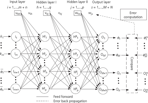
In the present study, a BPNN has been employed as an implicit mapping between the input parameter space and the space of responses at observation points. Figure 1 illustrates the general schema of a BPNN in which there is an input layer, two hidden layers and an output layer. The number of neurons in the input layer (I) is determined by the number of input parameters, which is herein the size of K(m). The number of output layer neurons (O) also depends on the number of reading points (M + N). The number of neurons in the intermediate hidden layers (HI, HII) that determine the main structure of the neural network and will have the most significant effect on the training method and overall performance of the network is determined through minimising a predefined error function on the training data by trial and errors.
In order to achieve the input data set of training data, different permeability combinations, which are determined by the OD method, are used. The output data set of the training data is obtained using information of the FE analysis at observation points.
As shown in Figure 1, in the network training, the data are first released forward (solid lines), and then the error values are calculated and returned backwards, and therefore the weight values at the connection points are corrected and updated (dotted lines). Here, the sigmoid transfer function is used as the transfer function, and thus all the training data are mapped linearly to the interval (0·1–0·9) before being placed in the input layer (Kurtulus and Razack, 2007). Moreover, the Levenberg–Marquardt learning algorithm is used in the back-propagation network for the training (Rafiai et al., 2013).
Genetic algorithm
GA, which has been used greatly in the past as an optimisation method, is used to solve many hydrological problems related to groundwater or surface water (Bastani et al., 2010; Karpouzos et al., 2001; Ko et al., 2012; Samuel and Jha, 2003). The GA is used to find the optimum permeability combination through which the objective function introduced in Equation 1 is absolutely minimised, and as a result, the best compatibility is achieved between the readings of instruments and the responses obtained from the neural network. To do this, a primitive population is first created randomly, each member of the population being a state of permeability combinations in different elements; then, the operators of the GA are performed sequentially, including the selection operator, cross-over operator, migration operator and mutation operator.
Introducing the characteristics of Baft earth dam
Specifications of Baft dam site
The Baft earth dam, which has a clayey core, is constructed on the Baft River, one of the branches of the Dahouj River, 160 km south-west of Kerman City in Kerman Province, to supply drinking water for Baft and Bezenjan and to control the floods of the river. Figure 2 illustrates an image of the overall view of the dam and its geographical location.
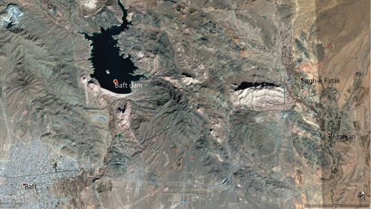
Overall view of the dam and its location. Image © 2017 DigitalGlobe. © 2017 Google
Overall view of the dam and its location. Image © 2017 DigitalGlobe. © 2017 Google
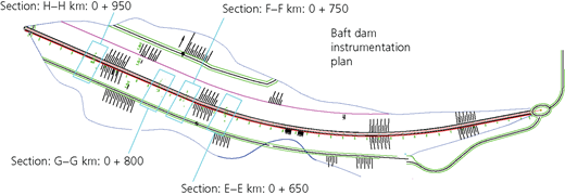
The dam catchment area is 259 km2, and the volume of the reservoir at the normal level of 2352·75 m above sea level is 40 million m3. The dam crest length is 1160 m, and its width is 10 m. The dam height is 65 m from the base, and its base width is 227 m in the largest cross-section. It is located at latitude 29°15′30″ north and at longitude 56°37′50″ east in the Jazmurian watershed. The general plan of the dam and its position are displayed in Figure 3.
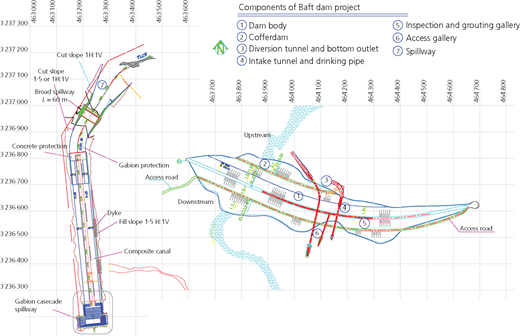
As shown in Figure 3, the river direction in the dam body is north–south and the axis of the dam is located ahead of the strait of the river, in a section with a direction of 195°. The main composition of the dam site includes five different parts; their characteristics, from the right-hand to the left-hand side, are as follows
the right-hand side bearing on limestone outcropping with a slope of 30° and a level of 2440 m above sea level
the smooth right-hand slope that is 210 m long, including surface dirt and weathered deposits with a thickness of 3 m; in this part, the dam body after excavating the surface layers is placed on the lower blend
the middle part including flood deposits with a thickness of approximately 10 m; the width of the river in this part is 4 m, and the floor of the river is 2295 m above sea level
the limestone section that is thin at first and then its thickness increases, with a length of 335 m below the dam body
the left arm, which is made up of alluvial deposits with a thickness of 2–6 m and a lowest point of 25 m below the dam crest and a length of 380 m.
In general, the deposits below the dam axis are a type of sedimentary rocks, which are extremely hard and resistant if they are not weathered or altered, and their compressive strength is more than 150 MPa. However, in the area below the dam, these rocks have become weathered and altered. The permeability of these rocks is very low (impermeable), which is very suitable for the reservoir and foundation of the dam. In general, excavation of alluvial deposits and strengthening of the weathered layers are considered for the sealing base of the dam. The general section of the dam body along with different parts of it is shown in Figure 4.
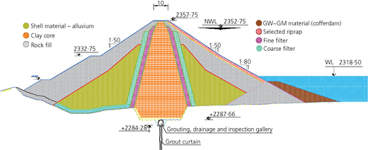
Typical section of Baft earth dam. Dimensions are in metres. GM, silty gravel; GW, well-graded gravel; NWL, normal water level; WL, water level
Typical section of Baft earth dam. Dimensions are in metres. GM, silty gravel; GW, well-graded gravel; NWL, normal water level; WL, water level
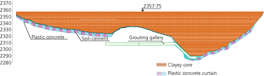
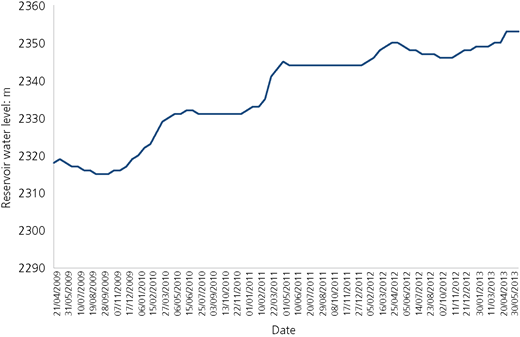
As can be seen, the clay core is in the central part and the fine- and coarse-grained filters are on its sides, and so is the shell of the dam. To protect the shell, the rock-fill cover is applied onto it, and on the upstream side there is also a riprap layer on it. Moreover, there is a water seal wall of plastic concrete in the weathered layer below the dam body. Figure 5, which shows the longitudinal profile of the dam embankment, indicates how the sealing wall is applied along the dam. Table 1 summarises the properties of the different parts of the dam used in its modelling. All specifications are derived from the results of the preliminary studies and design reports. The construction operation began after the completion of the preliminary studies in August 2003 and ended in September 2010. Dam impounding began in December 2008 and by May 2009 the level of water in the reservoir had risen to the level of 2318·97 m. However, since June 2009, some of this water has been released for agricultural uses and by October 2009 the level of the reservoir water had descended to 2314·68 m. Repeatedly, with the start of the water season in 2009, the level of water began to increase and eventually the water level in 2013 reached the level of 2352·75 m.
Specifications of different parts of the dam body
| Density: kg/m3 | Young’s modulus: MN/m2 | Permeability in x direction: m/s | Permeability in y direction: m/s | Cohesion: kN/m3 | Friction angle: ° | |
|---|---|---|---|---|---|---|
| Foundation | 2300 | 500 | 1 × 10⁻⁷ | 1 × 10⁻⁷ | 250 | 21 |
| Core | 1900 | 10·75 | 3 × 10⁻⁸ | 6 × 10⁻⁹ | 80 | 18 |
| Filters | 1900 | 37 | 1 × 10⁻⁵ | 1 × 10⁻⁵ | 7 | 37 |
| Shell | 1900 | 10 | 1 × 10⁻³ | 1 × 10⁻³ | 3 | 45 |
Characteristics of the instrumentation and measurement systems
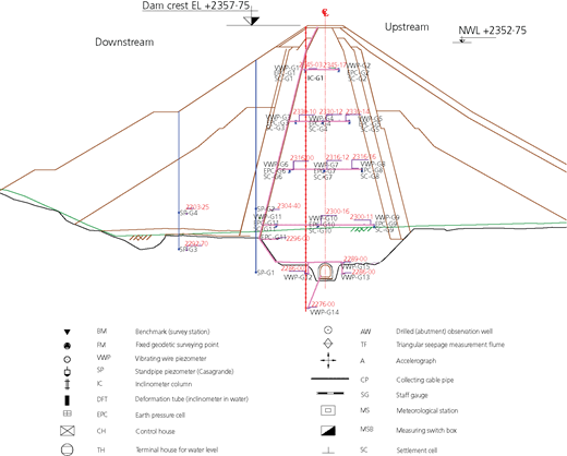
Continuous performance inspection of dams, in particular earthen dams, is important not only for recognising the behaviours of different parts of the dam but also from the safety point of view and for elimination of possible defects that may lead to dam destruction. Figure 6 displays different sections of the instrument implementations in the Baft dam where the modelling section of this study is shown as section G–G. Measurement tools include different kinds of piezometers, pressure gauges, seismometers, inclinometers, accelerometers and flowmeters. The exact location and alignment of their installation in section G–G are shown in Figure 7.
Inverse modelling of leakage in the Baft earth dam
Computational model structure
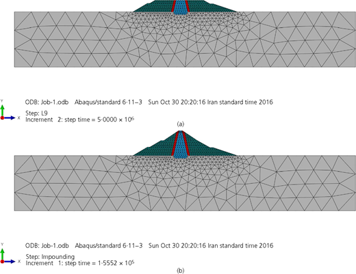
As previously mentioned, an FE model was made for the inverse leakage modelling in the G–G section of Baft earth dam shown in Figure 6. The constructed model consists of 1336 six-node triangular two-dimensional planar elements and 2781 nodes. All stages of dam construction and impounding have been modelled with regard to the actual time intervals. Figure 8 shows the model in the Abaqus software at two different stages, one at the time of body construction and the other at the start of the impounding stage. The variation in the water level in the lake behind the dam is shown in Figure 9; the impounding time intervals are actually considered in the modelling after the completion of the construction process for authenticity.
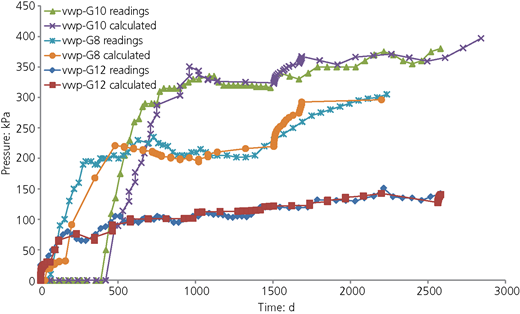
After completion of modelling and in order to validate the results, the pore water pressures obtained in some particular points were compared with actual values of readings of the piezometers. Figure 10 shows such comparison for the three vibrating wire piezometers G8, G10 and G12; their exact situations are displayed in Figure 7. The plausibly reliable fit between the results obtained from the FE model and the actual results in different parts of the dam, whether in its body or in its foundation, indicates the suitability of the model for use in inverse analysis.
Defining the variable space
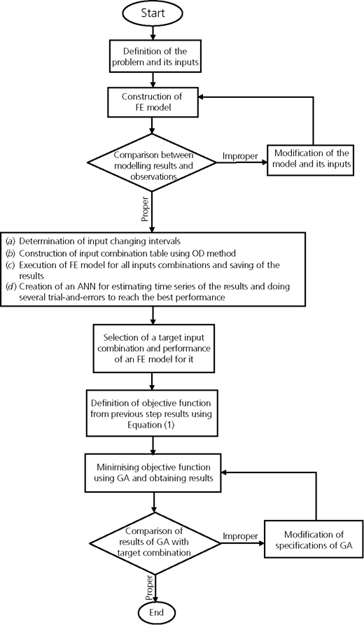
The first step in the inverse modelling process is to determine specifications of the model that are inconsistent and so could be effective in the leakage problem. Behaviour controls and analysis carried out during construction, impounding and operation of the Baft earth dam are all indicative of its proper performance and accurate design. However, in order to evaluate the applicability of the proposed method in inverse leakage modelling, in a group of elements the permeability has been conceptually changed; and then by assuming that the locations of these elements are indistinct, according to the obtained results from the FE model, in particular hydraulic heads and flow discharge rates, the locations of the elements has been searched. The general flow chart of the proposed method used in this study is displayed in Figure 11.
For a better assessment, regarding the results of the preliminary experiment sand studies that were available in the design reports, a domain of permeability variations has been determined for different parts of the dam and so some different states has been defined for the dam leakage analysis through the OD method. Table 2 displays permeability change intervals in different parts of the dam model.
Permeability change intervals in different parts of the dam body
| Region | Foundation | Core | Filters | Shell |
|---|---|---|---|---|
| Upper limit: m/s | 5 × 10⁻⁷ | 5 × 10⁻⁸ | 1 × 10⁻⁴ | 1 × 10⁻² |
| Lower limit: m/s | 1 × 10⁻⁸ | 1 × 10⁻⁹ | 5 × 10⁻⁶ | 5 × 10⁻⁴ |
As shown in Table 2, in view of the fact that permeability in the clayey core is very small, the amounts of permeability in both of its directions have been considered equal. In addition, with regard to the permeability variation intervals in different parts of the dam, seven permeability levels have been considered for each part as shown in Table 3. These permeability levels have been applied in the creation of an OD table L49 (76). Consequently, a set of 49 different permeability combinations has been made to be run in the FE model. In order to increase the efficiency and accuracy of the model, the foundation part has been divided into three sections as shown in Table 3.
Factors and levels used in OD selection: m/s
| Level | Foundation below the dam to 10 m depth | Foundation in depth between 10 and 20 m | Foundation below 20 m depth | Core | Filters | Shell |
|---|---|---|---|---|---|---|
| 1 | 1 × 10⁻⁸ | 1 × 10⁻⁸ | 1 × 10⁻⁸ | 1 × 10⁻⁹ | 5 × 10⁻⁶ | 5 × 10⁻⁴ |
| 2 | 2 × 10⁻⁸ | 2 × 10⁻⁸ | 2 × 10⁻⁸ | 2 × 10⁻⁹ | 1 × 10⁻⁵ | 1 × 10⁻³ |
| 3 | 4 × 10⁻⁸ | 4 × 10⁻⁸ | 4 × 10⁻⁸ | 4 × 10⁻⁹ | 2 × 10⁻⁵ | 2 × 10⁻³ |
| 4 | 8 × 10⁻⁸ | 8 × 10⁻⁸ | 8 × 10⁻⁸ | 8 × 10⁻⁹ | 4 × 10⁻⁵ | 4 × 10⁻³ |
| 5 | 1·6 × 10−7 | 1·6 × 10−7 | 1·6 × 10−7 | 1·6 × 10−8 | 6 × 10⁻⁵ | 6 × 10⁻³ |
| 6 | 3·2 × 10−7 | 3·2 × 10−7 | 3·2 × 10−7 | 3·2 × 10−8 | 8 × 10⁻⁵ | 8 × 10⁻³ |
| 7 | 5 × 10⁻⁷ | 5 × 10⁻⁷ | 5 × 10⁻⁷ | 5 × 10⁻⁸ | 1 × 10⁻⁴ | 1 × 10⁻² |
Defining the objective function
Time series related to the measurement of hydraulic heads and the flow discharge rates are required to construct the objective function. In this research, in order to obtain the objective function, hydraulic head time series of the points in the model corresponding to the actual location of the four piezometers G7, G8, G10 and G12, according to Figure 7, as well as the flow discharge rate time series in whole of the model, have been used.
In this way, at the start, a special permeability combination has been selected as the objective combination of the problem and the time series of hydraulic heads in the mentioned piezometers and flow discharge rate associated with this particular state have been obtained. Table 4 shows the permeability values in two objective combinations in the present study. Therefore, the purpose of inverse analysis is to find these permeability combinations according to the values of hydraulic heads in the locations of the G7, G8, G10 and G12 piezometers and the flow discharge rates of the dam. In other words, it is assumed that the time series of the responses are obtained from the readings of the piezometers and flowmeters over the time, and by having them, one would like to obtain the permeability values in different parts of the dam to compare them with the values considered in the design. Therefore, having the response values, through each FE analysis the time series of the hydraulic heads and the total flow discharge rates and consequently the value of the objective function (the value of f in Equation 1) could be obtained for each combination. Obviously, in the ideal case, the value of the objective function would be zero.
Inverse analysis in Baft earth dam
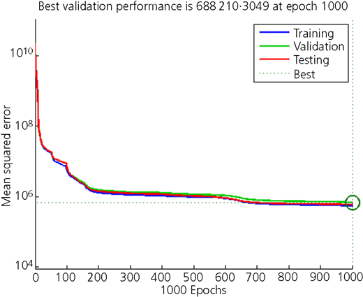
In order to perform the inverse analysis, the value of the objective function must be minimised. Thus, first, an ANN is constructed that can be used for any arbitrary combination of permeability to give the values of the hydraulic heads, as well as the total flow discharge rate at any time. In order to train such a neural network, the answers obtained through 49 iterations of FE analysis of the problem with different permeability combinations derived from OD have been used. The total number of training data is 7058 categories, which are related to different times, of which 10% has been used for testing, 5% for validation and the remainder for training. To determine the number of layers and the number of neurons in each layer, a large number of neural networks have been constructed, trained, tested and validated. A BPNN with four internal layers of, respectively, 8, 35, 15 and 5 neurons, had the best performance. Figure 12 shows the performance of this neural network during its training, testing and validation. As shown in this figure, the mean squared error of differences between actual results and the results obtained from the neural network is used to evaluate the performance.
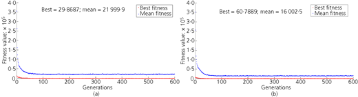
Finally, the GA has been used to minimise the objective function, where after so many iterations of trial and error, the initial population of 5000 individuals with probabilities of 85, 5 and 10% of cross-over, mutation and migration, respectively, has shown the best end results. Figure 13 shows its performance in different generations and the final answers which have been obtained after 600 generations are displayed in Table 5.
Permeability values obtained from reverse analysis: m/s
| Region | Foundation below the dam to 10 m depth | Foundation in depth between 10 and 20 m | Foundation below 20 m depth | Core | Filters | Shell |
|---|---|---|---|---|---|---|
| Case 1 | 5·0155 × 10−8 | 2·0325 × 10−7 | 5·0190 × 10−8 | 6·0046 × 10−8 | 1·8355 × 10−5 | 5·000 × 10−3 |
| Case 2 | 3·0023 × 10−8 | 1·0087 × 10−8 | 0·9983 × 10−7 | 3·9823 × 10−8 | 7·7459 × 10−5 | 1·0001 × 10−4 |
Conclusion
In this research, an inverse analysis method was proposed to find the flow characteristics of a dam (particularly the permeability of its different parts), taking into account the transient flow state and using the time series of hydraulic head changes and flow rate in the construction of the objective function. The proposed method is based on the use of FE analysis and combination of the ODs, ANNs and genetic optimisation algorithms that significantly reduce the volume of computations and increase the speed of solving large-scale real-world problems in engineering.
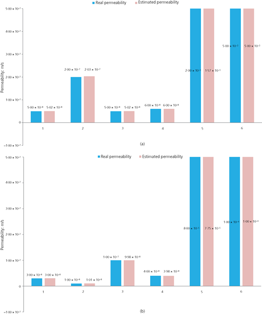
To investigate the efficiency of this method in solving real problems, the inverse analysis method was used to estimate the permeability of different parts of the Baft earth dam for two different permeability combinations, and very fine results were obtained. Figure 14 shows the comparison chart of the target permeability values and the estimated values from the proposed inverse analysis method for two different manners.
Comparison of obtained permeability and actual values: (a) first manner; (b) second manner
Comparison of obtained permeability and actual values: (a) first manner; (b) second manner
As shown in Figure 14, in all parts of the model, the results obtained from the inverse analysis are consistent with the intended values and only results in the area of the filters were slightly different from the actual results, which is negligible.
The obtained results indicate the possibility of using the proposed method in locating unconventional leakage in geohydraulic problems and assessing the weakness of a sealing system. Certainly, in order to improve accuracy and to find the location of the fault more precisely, it is possible to increase the number of divisions in modelling and have a more accurate evaluation for the treatment operations.
Although the present research shows the ability of the proposed method to perform an inverse analysis, some imperfections such as ignoring the variable nature of parameters, the effect of embankments and excavations on the permeability of the bed layers and the effect of climate change on effective parameters should be referred to (Huang and Rudnicki, 2006; Johnson, 1967), which are not considered in the modelling to simplify the problem and which can be used to conduct more accurate studies in future.

