

This paper provides guidance on quantifying the extent of corner effects in excavations and their impact on damage assessment. The corner effects’ extent is of great importance in making early decisions during project planning and preliminary design, particularly in relation to stakeholder engagement and placement of instruments. By using empirical relations, one is able to provide an equation, validated against the literature and additional numerical models, for estimating the extent of corner effects for a particular excavation geometry. Furthermore, two more equations for quantifying the damage of excavations to adjacent structures are presented and validated against two case studies in the literature. The proposed equations are also useful in the context of early stages of project development. Finally, a simple study shows the different effects of corners in sections parallel and perpendicular to a retaining wall. This highlights that corner effects may actually induce additional damage due to the introduction of a movement gradient, as opposed to the common previous perception that assumed that they were always conservative as they reduced absolute movements.
Notation
- B
length of short side of an excavation in plan
- dmax
distance from the corner of the excavation to the point where 90% of the maximum movement behind the wall occurs
- H
excavation retained height
- L
length in plan of the long side of an excavation
- δ2D
maximum lateral movement of the wall calculated using two-dimensional simulations
- δ3D
maximum lateral movement of the wall calculated using three-dimensional simulations
- δcorner
wall or ground movement at the location of the corner
- δmax
maximum lateral movement of the wall
Introduction
Corners affect the distribution of ground movements behind an excavation, as demonstrated extensively in the literature (e.g. Finno and Roboski, 2005; Finno et al., 2007; Fuentes and Devriendt, 2010; Hong et al., 2015; Hsiung et al., 2018; Lin et al., 2003; Moormann and Katzenbach, 2002; Ou et al., 2000; Roboski and Finno, 2006; Tan et al., 2014; Zradkovic et al., 2005). However, less work has been published on their effects on damage assessment on their surroundings (Finno and Roboski, 2005; Finno et al., 2007; Roboski and Finno, 2006) despite this being a critical consideration in the design and construction of excavations.
The most accurate way to approach damage assessment is using three-dimensional (3D) sophisticated numerical models that can cope with all of the complexities of behaviour surrounding an excavation. A two-dimensional approach (2D) can clearly not cope with corner effects without additional empirical considerations. However, at early stages of projects, particularly during planning or outline design, the 3D approach may be both time-consuming and expensive, and the 2D is only an approximation.
Therefore, a simple, economic and reliable approach that can obtain an early estimation of the extent and impact of corner effects on building damage assessment is of great value for practising engineers.
This paper presents a short literature review of previous work where the impact of excavation geometry was considered in relation to corner effects. Using validated published empirical methods, a relationship is derived and compared against case studies to show the extent of corner effects for different excavation geometries. This expression is critical to allow a final presentation of a formulation that allows building damage assessment to be estimated very simply that can be used by practising engineers. The paper finishes with a comparison of the inclusion of corner effects against ignoring them in building damage assessment and highlights their importance and relevance for structures with various positions and orientations with respect to the corners.
Effect of excavation geometry on corner effects
An interesting concept used in the literature to evaluate the effect of excavation geometry in the presence of corner effects is the plane strain ratio (PSR), which was firstly introduced by Ou et al. (1996) based on numerical analysis. PSR is defined as δ3D/δ2D, or the ratio between the maximum lateral movement of the wall, δmax, calculated using 3D simulations (δ3D) and 2D simulations (δ2D). PSR can be used as a proxy for the presence of corner effects by assuming that when PSR is lower than 1·0, corner effects must be present.
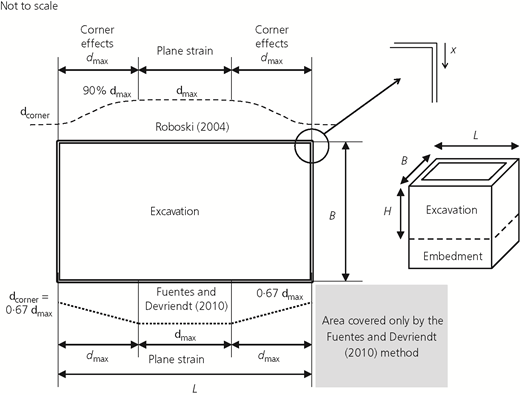
Figure 1 shows the excavation geometry nomenclature that will be used throughout the paper, where L is the length in plan of the long side of an excavation, B is the length of short side and H is the retained height.
Using the PSR approach, Moormann and Katzenbach (2002) found that excavations with an L/H ratio greater than 4·0 exhibited a PSR value of 1·0: in other words, corner effects were not evident at the centre of excavations. Finno et al. (2007) carried out similar work and estimated a value of L/H greater than 6·0 instead; they also showed that PSR reduces very rapidly when L/H is lower than 2·0.
In terms of the effect of the width of the excavation, Finno et al. (2007) showed that the effect of width was minimal for values of L/B greater than 2·0, while Lin et al. (2003) suggest values of L/B greater than 3·5 and Faheem et al. (2004) a value of 6·0. Tan et al. (2014) analysed multiple metro stations in Shanghai and observed only small variations for a large range of L/B values from ∼2 to ∼20. Other authors (Hsiung et al., 2018; Ou et al., 1996) have also shown that for increasing values of L/B, the PSR value also increases generally. In general, although they do not agree on a single limiting value of L/B, all indicate that for narrower excavations, the 2D wall displacement predictions in the longer wall are more accurate than for wider excavations if the same retained height is considered.
In summary, the preceding contributions indicate that, as a lower bound, 2D calculations provide similar results to 3D calculations in the estimations of δmax, for excavations where L/H is greater than 4·0–6·0, and L/B is greater than 2·0–3·5. For excavations with lower L/H and L/B ratios, the presence of corner effects is therefore assumed. Although all contributions seem to agree in that corner effects occur for all excavations, less agreement, and very little guidance, emerges when considering their extent.
Extent of corner effects
The use of empirical relations allows the extents of corner effects to be calculated simply and, when combined with case studies, provides confidence in their relationships. Two main methods are used here: the Roboski (2004) and Fuentes and Devriendt (2010) (F&D) methods.
Roboski (2004) introduced an ingenious use of the complementary error function (erfc) to model the ground movements (both horizontal and vertical) behind an excavation in a section parallel and along the wall (see Figure 1). For the remainder of this paper, the author uses movements meaning both horizontal and vertical ground movements, unless specified, because the empirical methods used here were validated for both. The method of Roboski (2004) was calibrated against different case studies in different ground conditions and provided satisfactory results for both horizontal and vertical ground movements. This method is fully summarised and further validated by comparison to an excavation in Chicago, USA, by Roboski and Finno (2006).
Equation 1 shows the horizontal movements behind an excavation wall (Finno and Roboski, 2005)
where x is the distance from the corner along the wall in plan (see Figure 1).
From Equation 1, the ratio of movement at any point along the wall is
from which it follows that at the corner where x = 0
which is only a function of the excavation geometry expressed as the ratio L/H.
Finno and Roboski (2005), through the use of the proposed function shown in Equation 1, inherently admit that a constant lateral movement of the wall (defined herein as plane strain) occurs in all cases. This is due to the function’s shape that is used to approximate the movements.
Equation 2 allows calculation of movements for each ratio of L/H and, therefore, the distance to plane strain movements can be observed. In order to have a consistent framework for comparison to cases from the literature, the author defines the distance to plane strain movements, x = dmax, as the distance from the corner of the excavation to the point where 90% of the maximum movement behind the wall occurs (see Figure 1). The value of 90% was selected somewhat arbitrarily to allow for a 10% variation around the maximum value. However, checks were made and taking another percentage level between 80 and 90% changes the figure only slightly and does not affect the process and results. It is important to note that a value between 90 and 100% may produce different results although it would be less conservative. Since a value of 90% is used, this is not strictly plane strain, although the author uses plane strain for simplicity. Applying the aforementioned definition – that is, δcorner/δmax = 0·9, Equation 2 can be rewritten as
From Equation 4, it can be seen that the ratio dmax/L is independent of the absolute values of L, H and δmax (i.e. the value of dmax/L is unique for a given ratio of L/H). The same equation allows representation of the relationship between dmax/L and L/H with a logarithmic expression shown in Equation 5, which is also shown as a dashed line in Figure 2 for simplicity of use. For validation purposes, another logarithmic line was fitted to the observed points marked in Figure 2, independently of Equation 4, and gave close results with coefficients 0·0581 and 0·1341 for Equation 5.
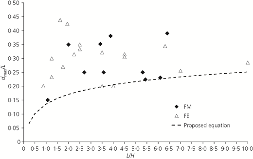
Position of plane strain movements for case studies and derived line. FE, finite element; FM, field measurement
Position of plane strain movements for case studies and derived line. FE, finite element; FM, field measurement
In order to investigate the adequacy of Equation 5, the case studies presented in Table 1 were observed for different values of L/H and are plotted in Figure 2, where FM stands for field measurement and FE for finite element, respectively, referring to the origins of the observations. The 12 FM case studies available from the literature in Table 1 were not sufficient to draw robust conclusions. Hence, additional case studies were created using an FE approach, the details of which can be found in the Appendix.
Details of case studies
| Case study (abbreviation) | Sourcea | FM/FE | Soil | Retained height H: m | Plan dimensions L × B: m × m | Corner angle: ° | Wall type | Construction method/propping system | δVmax approx.:b mm | δHmaxG/W approx.:c mm | dmaxH/V: m | dmax/L |
|---|---|---|---|---|---|---|---|---|---|---|---|---|
| New Palace Yard Car Park | Burland and Hancock (1977) | FM | London Clay | 18·5 | 66 × 50 | 90 | D-wall | Top-down/permanent slabs | 13 (e) 19 (s) | 30d | 12·5V (east) 16·5V (south) | 0·25 |
| Moorhouse | Zradkovic et al. (2005) | FE | London Clay | 40 | 35 × 35 70 × 35 140 × 35 | 90 | N/A | Bottom-up/multiprop (seven prop levels) | 22·5 31·0 38·0 | N/A | 7·0V 18·9V 28·0V | 0·2 0·27 0·2 |
| Immigration Building | Lee et al. (1998) | FM | Marine clay (soft, high plasticity) | 17·3 | 75·6 × 50·4 | 90 | D-wall | Bottom-up/multiple-level props | 110 | 60W | N/A | N/A |
| Taipei National Enterprise Centre | Ou et al. (2000) | FM | Silty clay (low plasticity overconsolidated) | 19·7 | 107 × 45 | 90 | D-wall | Top-down/permanent slabs | 78 | 25S 100W | 24V | 0·225 |
| 60 Victoria Embankment | St. John et al. (1993) | FE | Alluvium and London Clay | 19 | 67 × 29 | 90 | Secant pile wall | Top-down/permanent slabs | 28 | 34d,W | N/A | N/A |
| Basement 1 | Arup FE LS-Dyna results | FE | London Clay | 14·26 | 89·3 × 150 approx. | 90 | Secant pile wall | Top-down/horizontal temporary props in diagonal arrangement | 15·9 | 12·0 | 31 | 0·34 |
| Basement 2 | Arup FE LS-Dyna results | FE | London Clay | 15 | 24·4 × 29·2 (in one corner of the excavation) | 75 | Secant pile wall | Bottom-up/multilevel temporary corner props and horizontal prop | 7·8 | 8·9 9·3 | 10·7H 11·4H | 0·44 0·39 |
| Robert H. Lurie Medical Research Building (RLMRB) | Finno and Roboski (2005) | FM | Glacial clays (soft to stiff varying with depth) | 15 | 68 × 80 | 90 | Sheet pile | Bottom-up/tie-backs (three levels) | 80 (w) 60 (s) 50 (n) | 83W (w) 51W (s) 53W (n) | 17H (w) 18H (s) 32H (n) | 0·25 (w) 0·23 (s) 0·39 (n) |
| Takagi | Roboski (2004) | FM | Silt, peat and sandy and silty layers | 28 | 30 × ? | 90 | N/A | N/A | 52·5 | N/A | 4·5V | 0·15 |
| Chicago State Subway (Chi) | Finno et al. (2002) | FM | Sand overlying a thin stiff crust over stiff clays of increasing stiffness with depth | 12·2 | 47·3 | 90 | Secant pile wall | Bottom-up/tubular props and tie-backs | 40 | 38 | 18V | 0·38 |
| Flagship Wharf Building | Roboski (2004) | FM | Silt deposit, glacio-marine deposit and glacial till | 15·0 | 30 × 76 | 90 | D-wall | Bottom-up/three levels of tubular props | 28 | N/A | 10·5H | 0·35 |
| Frankfurt Clay | Moormann and Katzenbach (2002) | FM | Clay layered soil with sand bands and rocky limestone embedded | 15·8 | 34 × 54 | 90 | Secant pile wall | ?/tie-back at four levels | 175 | 175 | 17H | 0·31 |
| FE additional case studies | This paper | FE | Granular material overlying stiff overconsolidated clay | 12 | 30 ×30 30 × 15 15 × 30 42 × 42 54 × 54 54 × 27 27 × 54 84 × 84 | 90 | Shell element | Top-down | 2·89 2·75 0·67 4·14 4·97 4·10 2·90 6·30 | 3·80 3·08 1·10 5·6 6·8 6·0 3·7 8·5 | 10·0H 10·5H 4·5H 13·5H 16·5H 17H 8·5H 21·5H | 0·33 0·35 0·30 0·32 0·30 0·31 0·31 0·25 |
| FE additional case studies | This paper | FE | Granular material overlying stiff overconsolidated clay | 12 | 30 ×30 30 × 15 15 × 30 84 × 84 | 90 | Shell element | Bottom-up | 4·05 3·81 0·72 8·5 | 5·05 4·12 1·20 12·0 | 10·5H 10·5H 3·5H 23·5H | 0·35 0·35 0·23 0·28 |
Unless otherwise stated within the table and the notes below, all the information included in the table comes from the references listed in the second column
The letters inside parentheses in the last four columns represent the directions specified in the cited reference: e, east; n, north; s, south; w, west
The superscripts W and S represent whether the value was derived from observation of the wall or the soil, respectively
approx., approximate; FE, finite elements; FM, field measurement; H, horizontal movement; V, vertical movement
The proposed line constitutes a lower bound of the 26 case studies and was calculated by using the marked points for fitting. Figure 2 shows a significant scatter of points, with values of dmax/L ranging between 0·15 and 0·44. This means that between 30 and 88% of the wall length in plan is affected by corners. It also shows that for all the different conditions covered in the case studies, plane strain conditions occur (i.e. dmax/L < 0·5), confirming what was shown by other authors using the PSR method and the empirical methods of Roboski (2004) and Fuentes and Devriendt (2010). Equation 5 could be hence used as a conservative estimate of the position of plane strain movements, dmax, in an excavation.
Having the value of dmax is of double practical relevance to understand the extent of corner effects, because it allows the calculation of indicative levels of damage assessment at a very early stage of projects and also the decision of where to install monitoring stations to capture this phenomenon.
Building damage assessment: results and discussion
Traditionally, methods for establishing damage assessment have been based on the theories presented by Burland et al. (1977) and Boscardin and Cording (1989). These frameworks have been revised over time by many, such as Burland (2001), Cording et al. (2001) and Son and Cording (2005), but the variables used for the different assessments remain the same as in Figure 3. The Burland et al. (1977) method combines deflection ratio and horizontal strain to produce charts that provide guidance on the level of damage that a building is undergoing. Boscardin and Cording (1989) arrive at similar results using angular distortion and horizontal strains instead.
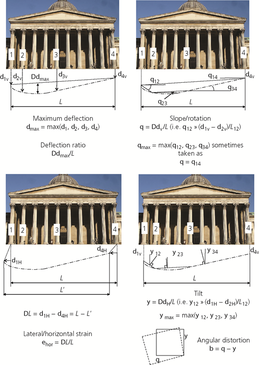
As shown earlier, the main focus has been on the combination of horizontal strain and either angular distortion or deflection ratio. This section of the paper focuses on the deflection ratio and angular distortion as they are immediate results of both empirical methods’ formulations.
Roboski and Finno (2006) proposed Equation 6 to estimate the maximum slope/rotation (as defined in Figure 3) parallel to the wall. It must be noted that Roboski and Finno used the term ‘distortion’ as opposed to ‘slope/rotation’, and in doing so, were assuming that tilt was zero.
A similar equation, Equation 7, can be derived for the method proposed by Fuentes and Devriendt (2010), when combining it with the derived dmax in Equation 5. Due to the method’s assumption, rotation, angular distortion and deflection ratio are all equal for zero tilt (see Figure 3).
The value of 0·33 in Equation 7 comes from the assumption that δcorner/δmax = 0·67 as recommended by Fuentes and Devriendt (2010). However, the use of another ratio – that is, using Equation 3 or another calibrated value – allows this to be adapted to other conditions, as will be shown later.
Both Equations 6 and 7 provide an estimate of maximum slopes in sections parallel to the retaining wall for both horizontal and vertical movements. Both also depend only on the geometrical parameters of the excavation and the maximum movement; close observation shows that, in fact, both are independent of the absolute values of L and H. This allows a simple and quick comparison of various geometries, as shown in Figure 4.
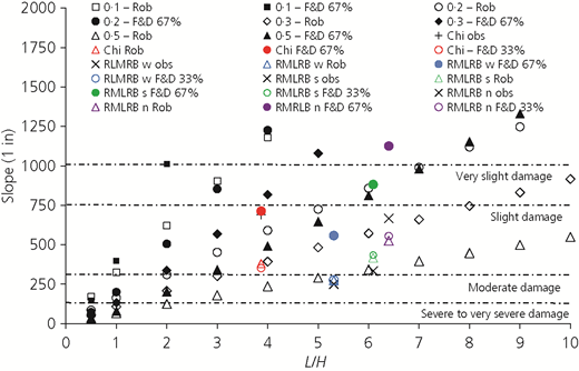
Slope against L/H estimation using both methods compared to two case studies (please refer to Table 1 for details of case studies shown). n, north; obs, observed; Rob, Roboski’s method; s, south; w, west
Slope against L/H estimation using both methods compared to two case studies (please refer to Table 1 for details of case studies shown). n, north; obs, observed; Rob, Roboski’s method; s, south; w, west
Figure 4 shows the results from both methods for different excavation geometries, L/H. The two methods differ in their predictions when a value of δcorner/δmax equal to 67% is used in the F&D method, although the differences are reduced significantly when this value is taken as 33%. The results from two sites are also included for validation purposes (see Table 1 for details). In the Chicago State Subway (Chi) site, a maximum slope in the direction parallel to the wall of 1 in 690 was observed for a basement with an L/H ratio of 3·87 and δmax/H of 0·33%, which agrees better with the prediction of the F&D method, 1 in 713, than that of the Roboski method, 1 in 347 (underestimated by almost 50%). Conversely, the data presented for the Robert H. Lurie Medical Research Building (RLMRB) excavation shows the opposite trend. Here Roboski’s method provides a much better fit to the measurements than that presented by Fuentes and Devriendt for a value of δcorner/δmax equal to 67%, although the match is similar when this value is chosen as 33%.
Figure 5 shows a similar graph for increasing maximum movement behind the wall. As expected, the slope reduces with increasing movement. It indicates that for values of δmax/H (%) greater than 0·3 and any values of L/H up to 10·0, the values of slope are normally close to 1 in 1000, which would traditionally constitute a warning level for many structures as incipient ‘very slight damage’ – for example, as presented by Boscardin and Cording (1989). The dashed lines in Figures 4 and 5 show the damages thresholds for angular distortion for a lateral strain equal to zero as recommended by Boscardin and Cording (1989).
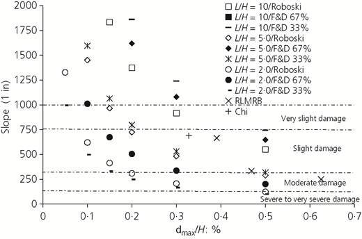
Slope against δmax/H estimation using both methods compared to two case studies
Slope against δmax/H estimation using both methods compared to two case studies
For lower values of L/H, close to 2·0, the slope reaches concerning levels for lower values of δmax/H (%). This means that for excavations with shorter walls (lower values of L/H), more potential for damage is predicted for the same retained height and maximum movement. This is because the movements need to accommodate a similar total change over a shorter distance. The RLMRB values seem to fall within the range of values calculated by both methods for L/H = 5 when using the Roboski and F&D methods with a value of 33% for δcorner/δmax. A similar agreement is observed for the Chi case study which has a value of L/H equal to 3·87.
The preceding discussion confirms that both methods provide similar values of building damage but that a value of δcorner/δmax = 0·33 seems to provide more accurate results despite the value of 0·67 that was recommended by Fuentes and Devriendt (2010).
The relevance of being able to use the F&D method with confidence is that it allows damage assessment to be calculated in the shaded area of Figure 1, which has not been demonstrated for other empirical methods. Hence, the remainder of this section covers additional analyses that were carried out using the F&D method only.
These extra analysis cases are shown in Figure 6 and were done as building damage assessment. The figure shows an excavation of dimensions 100 m × 50 m and 15 m deep and 13 simulated buildings for which damage assessment was calculated using two options, considering corner effects and not considering them.
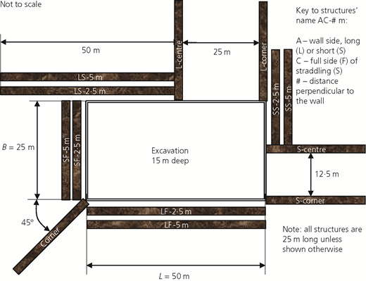
Parallel to the wall, buildings were placed along the long side of the wall covering the full length and the short length and straddling the corner. Perpendicular to the wall, buildings were placed at the centre and at the corner of excavations on both sides. A final building was placed in the corner of the excavation at a 45° angle. It must be noted that the problem is fully symmetrical.
The analyses were run in the software Oasys Xdisp 19.4 (Oasys, 2016) where the F&D method is implemented. A value of δcorner/δmax = 0·33 was used and dmax, necessary for the calculations, was estimated using Equation 5, giving the values of 8 and 3·64 for the long and short sides, respectively. The building damage assessment criteria follow the limits established by Burland (2001): negligible (N), very slight (VS), slight (S), moderate (M) and severe (SE), with transition values of horizontal ground strain between zones of 5 × 10⁻⁴, 7·5 × 10−4, 1·5 × 10−3 and 3 × 10⁻³.
Two ground deformation profiles were used for input as shown in Figure 7: one with a large movement using the Taipei National Centre (Ou et al., 2000) and another with smaller movements using the House of Commons site (HOC) (Burland and Hancock, 1977). These deformation profiles are necessary for the F&D method and describe the deformation of the ground in a cross-section perpendicular to the wall at the centre as shown by Fuentes and Devriendt (2010).
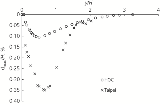
Table 2 summarises the interesting results. For small deformations – that is, HOC where δmax/H (%) = 0·1 – the consideration of corner effects reduces the level of damage around the corners in sections perpendicular to the wall. In all other cases, the damage is negligible due to the small movements. This shows the potential savings of including corners for structures around corners.
Building damage assessment results
| Taipei | HOC | |||
|---|---|---|---|---|
| With | Without | With | Without | |
| LF-2·5 m | N | N | N | N |
| LF-5 m | S | N | N | N |
| SF-2·5 m | S | N | N | N |
| SF-5 m | S | N | N | N |
| LS-2·5 m | S | M | N | VS |
| LS-5 m | S | M | N | N |
| SS-2·5 m | S | VS | N | N |
| SS-5 m | S | VS | N | N |
| L-centre | SE | SE | VS | VS |
| L-corner | S | SE | N | VS |
| S-centre | SE | SE | VS | VS |
| S-corner | S | SE | N | VS |
| Corner | S | M | N | N |
For larger deformations – that is, Taipei, where δmax/H (%) = 0·35 – the behaviour is more complex. For sections parallel to the wall, the inclusion of corner effects increases the level of damage for almost all structures and, therefore, is not conservative. In the perpendicular direction, the differences are also significant near the corners. When corner effects are not considered, the damage level is severe for all sections, except the bisector section which is moderate. Conversely, including corner effects reduces the level of damage at the corner and the bisector significantly.
Table 2 shows the importance of considering the corner effects but highlights how both sections parallel and perpendicular to the wall must be considered at the same time and how the behaviour may vary for different magnitudes of ground movements.
Conclusions
All excavations presented in the literature and studied in this paper present corner effects as defined here. However, for excavations where L/H is greater than 4·0–6·0 and L/B is greater than 2·0–3·5, these can be neglected in terms of the estimation of the maximum movement, although this does not mean corner effects do not exist.
The extent of corner effects, expressed as the distance from the corner, is important for making early decisions about the potential impact of an excavation on surrounding buildings, as well as helping to decide the location of instrumentation. A conservative relationship validated against 26 case studies has been provided.
The earlier-mentioned relationship also allows the estimation of maximum slope, as an indicator of potential damage, which can be estimated easily using two equations. One requires an estimate of the maximum movement and the other requires the ratio between corner and centre movements to be used.
Furthermore, the inclusion of corner effects in damage calculations can have very different implications whether considering sections parallel or perpendicular to the wall in plan. For large ground movements δmax/H (%) = 0·35, the damage increases in sections parallel to the wall but reduces in areas near the corner for perpendicular sections when comparing it to the case of not considering corner effects. In the cases of small movements, δmax/H (%) = 0·1, the damage is lower when including corner effects for both directions. This highlights the importance of considering corner effects and also both directions.
Appendix: three-dimensional FE modelling: additional case studies
A parametric study was undertaken using a 3D FE model. The parametric study consisted of different combinations of the L/H and L/B ratios. The choice of these parameters is based on the findings of Finno et al. (2007) and Moormann and Katzenbach (2002), who showed these to be the most relevant parameters.
A computer program called HyperMesh v. 10·0 (Altair, 2009) was used to create the mesh and the topology of the problem, while LS-Dyna (LSTC, 2008) was used to undertake the numerical analysis of the problem.
Problem geometry and FE mesh dimensions
The retained height, H, was selected as 12 m throughout the study, and the excavation had a length L and a width B. The L/H ratios chosen were 2·5, 3·5, 4·5 and 7·0. This resulted in lengths of the wall, L, equal to 30, 42, 54 and 84 m. The values of L/B varied between 1·0 and 2·0. The problem is symmetric about the two axes that pass through the centre of the excavation; hence, only one-quarter of the excavation was modelled, as shown in Figure 8.
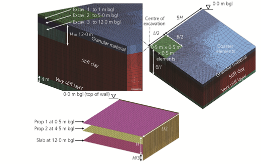
The retaining wall dimensions were also fixed to a width of 1·0 m and a depth of embedment of 4·0 m below final excavation level. The thickness of the wall was kept constant for all the different analyses, after the findings of Moormann and Katzenbach (2002), who showed that it has little influence on the movements and the corners. The excavation depth of the wall was also kept constant, following the conclusions of Zradkovic et al. (2005: p. 512): ‘The effect of the embedment depth of a wall on movements and structural forces in the excavations analysed is negligible’. Whittle and Hashash (1992) support this latter statement and concluded that the wall embedment has a negligible effect in ground and wall movements, particularly in situations of soil pre-failure.
Roboski (2004) recommended the lateral boundaries of the mesh to be placed at a distance of 5H from the retaining wall. Lin et al. (2003) showed that a distance of 3H to the boundary was sufficient. The recommendations of Roboski (2004) were adopted in this study to allow for a greater distance behind the wall over which to obtain ground movements free of boundary effects. The lower boundary of the problem was also located at a distance 5H from the bottom of the excavation.
The vertical boundaries of the mesh were restrained in the horizontal direction and free to move in the vertical direction. The bottom of the mesh was fixed in all directions.
The FE model was built using hexahedral and tetrahedral elements. The remainder elements accounted for less than 1% of the total number of elements.
Elements within the excavation were modelled with dimensions of 0·5 m × 0·5 m × 0·5 m. The rest of the elements outside this area varied in dimensions, with coarser elements appearing with greater distance from the excavation as shown in Figure 8.
Soil profile, material models and groundwater
The soil profile shown in Table 3 consisted of a layer of 5 m of granular material overlying stiff clay, similar to that taken by Grammatikopoulou et al. (2008), which represents a typical situation in the city of London. Underlying the clay, a 4 m, very stiff, granular material layer was used to provide a rigid boundary. Furthermore, Jen (1997) showed in a parametric study that the depth of overlying granular materials over an overconsolidated clay has a small influence in the ground movements, particularly when the top of the clay is above the excavation level; Yeow and Feltham (2008) confirmed this.
Soil stratigraphy and parameters
| Soil | Top of layer: m bgl | γ: kN/m3 | E′: GPa | φ ′ | K0 |
|---|---|---|---|---|---|
| Granular soil | 0 | 20 | 25 | 30 | 0·5 |
| Clay | 5 | 20 | See the paper of Fuentes et al. (2018) | ||
| Very stiff granular material | 68 | 20 | 150 | 36 | 0·41 |
The granular materials were modelled using a linear elastic perfectly plastic Mohr–Coulomb material. The clay was modelled using the non-linear small-strain stiffness model Brick developed by Simpson (1992). The validated ‘most probable’ parameters for Brick presented by Fuentes et al. (2018) were used. The parameters used for the simulations are presented in Table 3.
The groundwater table was placed 0·5 m below ground level (bgl) and followed a hydrostatic profile to the bottom of the problem.
Construction sequence
The same construction sequence was followed for all the different simulations. The type of analysis in terms of drainage is shown in parentheses for each stage in the clay. The remaining soils were granular materials and were always treated as drained.
Initialise (drained).
Wish in place retaining wall (undrained).
Excavate to 1 m bgl (undrained).
Install temporary prop at capping beam level and excavate to 5 m bgl (undrained).
Install temporary prop at level 2 and excavate to the formation level (undrained).
Install base slab (undrained).
Remove temporary prop at level 2 (for bottom-up construction sequence only) (undrained).
Support systems’ modelling and properties
Different construction sequences, top-down and bottom-up, were modelled by simply changing the stiffness of the temporary props used in the model. For the top-down construction, the stiffness of a concrete slab was used. For the bottom-up model, the stiffness was calculated using 660 mm external diameter circular hollow sections placed at 10 m intervals. This arrangement is typical of London, as shown by Fuentes et al. (2018).
The weight of the prop elements was reduced to a very small value to avoid imposing significant loading on the wall, which would be unrealistic. The base slab was, however, modelled with full weight as its effect on the behaviour of the formation level is important.
A stiffness of 2·1 × 107 kN/m2 (that of concrete in the short term) was used in the top-down case. The top two levels and the slab were taken as 0·3 m and 1·2 m thick, respectively.
In the bottom-up construction sequence, the tubular props mentioned earlier had a stiffness of 4·2 × 106 kN/m2 and a thickness of 0·4 m.

