A simple model for tertiary creep in geomaterials

Osman, Ashraf S; Birchall, Thomas J; Rouainia, Mohamed

doi:10.1680/jgere.19.00025

This paper presents a constitutive modelling approach for the viscoplastic-damage behaviour of geomaterials. This approach is based on the hyperelasticity framework, where the entire constitutive behaviour is derived from only two scalar potentials: a free-energy potential and a dissipation function. The novelty of the new proposed model, in addition to being thermodynamically consistent, is that it requires only a few parameters that can be derived from conventional laboratory testing. The model has been specifically tested for its ability to reproduce a series of triaxial compression tests on core rock samples. The comparison between the viscoplastic-damage model predictions and experimental results shows that the model is remarkably successful in capturing the stress–strain response both at peak stress and in the region of material softening and the time to reach failure.

Notation

A: total cross-sectional area of a surface within the unit cell
$A_{n + 1}^{(k)}$: algorithmic modulus
A_s: solid matrix area within A
C: friction angle
c₁: material parameter related to cohesion
c₂: material parameter related to the friction angle
c₃: material parameter related to the dilation angle
D: dissipation rate
D: viscoplastic-damage consistent tangent modulus
D^e: standard isotropic elasticity tensor
E: Young’s modulus
${\dot{e}}^{p}$: plastic deviator strain rate
F: Helmholtz free-energy function
f: yield function
G: shear modulus
I: second-order unit tensor
K: bulk modulus
k: iteration counter
m: order of the dissipation function D
n: material constant
p: effective mean stress
q: deviatoric stress invariant
r_d: material constant that governs the ratio of damage
r_p: material constant that governs the ratio of viscoplasticity
t: time
α_d: material damage occurring with a representative continuum volume element
α_p: micro-plastic strain
${\dot{α}}_{v}$: plastic volumetric strain rate
β: softening/hardening parameter
ϵ: total strain tensor
ϵ^e: elastic strain tensor
${\dot{ϵ}}^{p}$: plastic strain rate
ε_f: tolerance
ε_r: relative tolerance
η: viscous coefficient that controls the extent of plastic strain
Λ: arbitrary Lagrangian multiplier
ν: Poisson’s ratio
Π(α_d): hardening/softening function
σ: true stress tensor
φ: angle of friction
χ: generalised stress tensor
$\bar{χ}$: dissipative stress tensor
ψ: dilatancy angle

Introduction

Creep may be defined as continued deformation without a stress change. Creep has been studied since about 1905, although such behaviour was documented as early as 1833 (Griggs, 1939). Most early studies focused on the creep rupture of metals under tensile stress. However, later studies have been carried out on rocks, in particular salt rocks, as these soft rocks creep under temperature and stress conditions, as evidenced from laboratory data (Hayano et al., 2001). Determining the creep characteristics of rock is an important stage in developing a tool that can predict the time-dependent deformation of an underground cavity. Creep tests performed in the laboratory are very significant in mining and improved design of underground structures (Cristescu, 1989). Creep testing of rock in the laboratory has been carried out by a number of researchers (Heap et al., 2010; Langer, 1982; Le Comte, 1965; Li and Xia, 2010; Obert, 1965; Phueakphum et al., 2010; Scott-Duncan and Lajtai, 1993; Singh, 1975; Vouille et al., 1984; Yang and Jiang, 2010). The simplest creep tests are those during which the rock specimen is uniaxially loaded in compression. The testing procedure involves an increment of load applied quickly to the rock specimen, and the stress is held constant while the gradually increasing strain is recorded regularly (Goodman, 1989). Triaxial tests have also been carried out in which the sample is confined by an all-around pressure, more closely simulating in situ conditions. The duration of an individual creep test is generally several weeks or months. Tests lasting a number of years have also been reported (Cristescu, 1989).

Laboratory data from creep tests are mostly depicted in the form of strain–time curves of which the general form is displayed in Figure 1 (Goodman, 1989; Jaeger et al., 2007; Jeremic, 1994). An instantaneous elastic strain, ϵ_e, is followed by primary or transient creep (region 1) in which strain occurs at an ever-decreasing rate. Secondary creep (region 2) follows if the constant stress overcomes a given limit and is characterised by a constant strain rate. For higher constant stress levels, tertiary creep (region 3) is also observed, which is characterised by a strain rate increase with time and leads eventually to failure. As illustrated by Jeremic (1994), laboratory investigations have shown that removal of the applied load in region 1 at point P of Figure 1 causes the strain to decrease rapidly to point Q (change in strain equal to ϵ) and then asymptotically back to zero at point R. Thus, region 1 can be classified as viscoelastic. Removal of stress in region 2 at point T will result in permanent deformation (VO). Thus, region 2 can be classified as viscoplastic. Despite the classification of these regions as viscoelastic and viscoplastic being an idealisation, it is reasonable to think that at low levels of stress the material behaviour is roughly viscoelastic and at high levels the behaviour is viscoplastic. The tertiary stage of creep behaviour (region 3) appears due to progressive microcracking of the material and would result in a loss of strength and stiffness, which may eventually lead to failure and a complete loss of the load-carrying capacity of the material.

Figure 1

View large Download slide

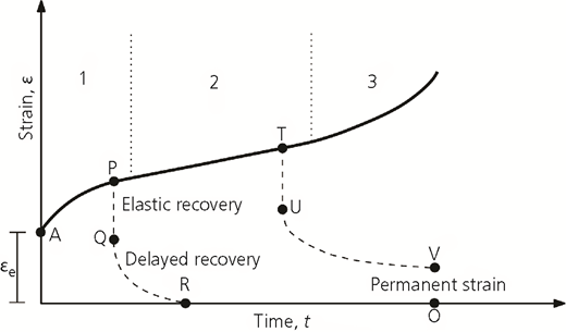
Typical deformation of creep materials as a function of time (after Jeremic (1994))

Creep behaviour can also be classified according to the acting stress; it is possible to divide creep behaviour into volumetric and deviatoric (or shear) creep (Tavenas et al., 1978). Volumetric creep is caused by constant volumetric stress, and deviatoric creep is caused by constant deviatoric stress. Generally, volumetric creep consists only of the primary phase of the creep deformation – that is, it tends to stabilise. Deviatoric creep may or may not consist of all three phases, depending on the shear mobilisation. If the deviatoric stress is low, then only the primary creep phase will appear, but after crossing some level of the shear mobilisation, the primary phase will be followed by the secondary phase, which can lead to the tertiary phase and creep rupture. Tertiary creep is often observed in soft rocks, and it represents a problem in a mining environment.

There are a great number of constitutive models developed to account for the time-dependent creep behaviour of geomaterials. Extensive reviews for constitutive modelling of creep can be found in the papers by Liingaard et al. (2004) and Grimstad et al. (2017). Existing constitutive models for creep behaviour can generally be classified into three categories (Liingaard et al., 2004): (a) elementary phenomenological models, (b) rheological models and (c) general stress–strain–time models.

In elementary phenomenological models, empirical relations are obtained by directly fitting the observed test data with simple mathematical functions. Logarithmic and exponential laws are often adopted to link creep strain to time. Examples of these models can be found in the papers by Singh and Mitchell (1968), Campanella and Vaid (1974), Leroueil (1987), Yin (1999) and Bi et al. (2019). One of the basic limitations of elementary phenomenological models is that they are strictly valid only for conditions that are identical to those of the test from which they were derived (e.g. one-dimensional (1D) condition). However, they can provide practical solutions to engineering problems, as far as the boundary conditions are consistent with the laboratory experiments.

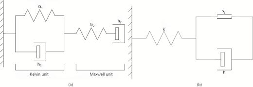
Rheological models consist of a combination of different components, such as springs, dashpots and sliders, to describe the time-dependent creep behaviour of a material. The structure of these models is not related to a particular creep test, and therefore, only the model parameters change between tests in order to provide a fit for the strain–time data. Linear viscoelastic models consist of various combinations of two states of deformation, elastic behaviour (represented by a spring) and viscous behaviour (represented by a dashpot). Many different linear viscoelastic models have been proposed, such as the Maxwell, the Kelvin and the Burgers model. The simplest model that can be used to trace strain up to the onset of secondary creep is the Burgers model, which is composed of a Maxwell model and a Kelvin model connected in series (Figure 2(a)). An overview of these viscoelastic models can be found in the book by Jaeger et al. (2007). These viscoelastic models are typically formulated for 1D problems. However, they can be extended and applied to three-dimensional boundary-value problems. Birchall and Osman (2012), for example, presented analytical solutions for predicting the creep displacements of deep tunnels in three dimensions using the Burgers model. Linear viscoelastic models cannot simulate the failure of geomaterials. Slider elements (St Venant elements) are added to the elastic and viscous components of viscoelasticity in order to include the failure process. Typically, a slider element is placed in parallel with a dashpot element, known collectively as a Bingham unit (Figure 2(b)). The model by Perzyna (1966) is a well-known example of a viscoplasticity model. A viscoplastic material exhibits a time-dependent behaviour only in the plastic region. This behaviour corresponds to the secondary stage of creep. However, these models cannot replicate tertiary creep behaviour.

Figure 2

View large Download slide

Examples of rheological models: (a) Burgers model; (b) Bingham model

Generalised stress–strain models can describe both viscous effects and rate-independent behaviour of soils under general loading conditions. Several theoretical approaches have been used to derive these models. Borja and Kavazanjian (1985), for example, used the concept by Bjerrum (1967) of total strain decomposition into an immediate (time-independent) part and a delayed (time-dependent) part to model the stress–strain–time behaviour of wet clays. A modified Cam-Clay yield surface (Roscoe and Burland, 1968) is employed to characterise the time-independent stress–strain behaviour. Kaliakin and Dafalias (1990) presented a bounding-surface model for the time-dependent response of overconsolidated soils. The basic characteristic of the bounding-surface approach is that the material exhibits a memory of the loading history and the plastic deformation depends on the distance between the present stress point and an image stress point on the bounding surface defined by a mapping rule for stress states within the surface. Hashiguchi and Okayasu (2000) adopted the subsurface modelling approach to simulate the time-dependent behaviour. This model assumes a bounding surface and a subloading surface that always passes through a current stress point. The model can describe the continuous stress rate–strain rate relation in the loading process with smooth elastic–plastic transition. Despite the complexity of the generalised models mentioned earlier, numerical investigations have focused on volumetric creep under undrained conditions, despite the fact that creep is an inherently drained phenomenon, as it takes a long time to develop (Jardine, 2014, Kavvadas and Kalos, 2019). At large shear stress approaching strength, deviatoric creep strain rates accelerate and lead to tertiary creep and failure (Bishop, 1966).

The literature on constitutive formulations for predicting tertiary deviatoric creep is sparse. Dragon and Mroz (1979), Al-Shamrani and Sture (1998), Pellet et al. (2005) and Shao et al. (2003) modelled tertiary creep using a strain-softening/hardening approach based on the shear-stress-driven damage mechanism. Gioda and Gividini (1996) predicted tertiary creep by introducing viscous damage on a Bingham model. Kavvadas and Kalos (2019) presented a time-dependent constitutive model for cohesive structured soils (TMS model). The TMS model is constructed from three characteristic surfaces: (a) an internal plastic yield envelope (PYE), which is a small surface bounding the elastic domain; (b) an external structure envelope (SE) bounding the PYE and all accessible states; and (c) an intrinsic envelope, corresponding to an equivalent intrinsic state. The size, shape and location of the SE give the magnitude of the structure (and strength), which increases with viscous volumetric strains and degrade with plastic strains and viscous shear strains. The TMS model is capable of simulating tertiary creep; however, it requires identification of 21 material constants.

The main aim of this work is to model tertiary creep using a sound theoretical framework. The new simple model, presented here, makes use of damage mechanics concepts. The damage mechanics framework is a powerful tool that can be used to simulate many features in geomechanics, as illustrated by Xiao and Liu (2017) and Xiao and Desai (2019a, 2019b). This paper extends the hyperplasticity approach of Collins and Houlsby (1997), Houlsby and Puzrin (2000) and Puzrin and Houlsby (2001) to model coupled viscoplastic-damage frictional materials. This paper focuses on deviatoric creep and presents a model that obeys the laws of thermodynamics. The entire constitutive behaviour can be derived from two scalar potentials: a free-energy potential that provides the elasticity law and a dissipation potential that provides the yield function, the direction of plastic flow and the evolution of a damage variable. No additional assumptions are required. The motivation here is to derive a simple model. Thus, the new model has only a few parameters that have physical meanings and is capable of capturing the tertiary creep observed in soft rocks.

The hyperplasticity framework

For isothermal deformations of a continuum undergoing small strains, the first and second laws of thermodynamics can be written as

σ : \dot{ϵ} = \dot{F} + D

1

where F represents the Helmholtz free-energy function; D is the dissipation rate, which is strictly non-negative; and σ denotes the true stress tensor and ϵ denotes the total strain rate tensor. Collins and Houlsby (1997) and Houlsby and Puzrin (2000) introduced the hyperplasticity theoretical framework, in which they demonstrated that the material behaviour can be determined from the knowledge of the two thermodynamic potential functions F and D. The local state of the material is assumed to be defined completely by the knowledge of (a) the strain tensor ϵ, (b) a set of internal tensor variables and (c) the entropy. For the isothermal case, the entropy does not enter into the formulation.

For a damaged material, the internal variables can, most usefully, be thought of as the micro-plastic strains α_p and the material damage α_d occurring within a representative continuum volume element. Therefore, free energy is chosen to be of the form F(ϵ, α_p, α_d), while the dissipation rate function is taken to be $D (\dot{ϵ}, α_{p}, {\dot{α}}_{p}, {\dot{α}}_{p}, {\dot{α}}_{d})$ ⁠. If the dissipation function is homogenous of the first order, then Equation 1 can be rewritten as

σ : \dot{ϵ} = \frac{\partial F}{\partial ϵ} : \dot{ϵ} + \frac{\partial F}{\partial α_{p}} : {\dot{α}}_{p} + \frac{\partial F}{\partial α_{d}} : {\dot{α}}_{d} + \frac{\partial D}{\partial {\dot{α}}_{p}} : {\dot{α}}_{p} + \frac{\partial D}{\partial {\dot{α}}_{d}} : {\dot{α}}_{d}

2

It follows that

σ = \frac{\partial F}{\partial ϵ}

3

and

\begin{array}{l} (χ_{p} - {\bar{χ}}_{p}) : {\dot{α}}_{p} = 0 \\ (χ_{d} - {\bar{χ}}_{d}) : {\dot{α}}_{d} = 0 \end{array}

4

where the generalised stress tensors χ_p and χ_d are given by

\begin{array}{l} χ_{p} = - \frac{\partial F}{\partial α_{p}} \\ χ_{d} = - \frac{\partial F}{\partial α_{d}} \end{array}

5

and the dissipative stress tensors ${\bar{χ}}_{p}$ and ${\bar{χ}}_{d}$ are given by

\begin{array}{l} {\bar{χ}}_{p} = \frac{\partial D}{\partial {\dot{α}}_{p}} \\ {\bar{χ}}_{d} = \frac{\partial D}{\partial {\dot{α}}_{d}} \end{array}

6

Following the orthogonality condition by Ziegler (1983), which was adopted in the hyperplasticity framework of Houlsby and Puzrin (2000), a wide range of classes of materials can be described by enforcement of the stronger condition in Equation 4

\begin{array}{l} χ_{p} = {\bar{χ}}_{p} \\ χ_{d} = {\bar{χ}}_{d} \end{array}

7

To develop rate-independent thermomechanical models, Puzrin and Houlsby (2001) suggested a decoupled form of dissipation function that is appropriate for multiple surface kinematic hardening plasticity models. For a rate-independent damage material, the dissipation function takes the form of

D = \frac{\partial D}{\partial {\dot{α}}_{p}} : {\dot{α}}_{p} + \frac{\partial D}{\partial {\dot{α}}_{d}} : {\dot{α}}_{d}

8

As noted by Einav et al. (2007), adopting a decoupled dissipation for rate-independent plasticity-damage models may result in damage prior to plastic straining or vice versa. Furthermore, the uncoupled dissipation potentials imply multi-yield surfaces, each one associated with the evaluation of each internal variable. Therefore, Einav et al. (2007) proposed a coupled dissipation function for rate-independent materials, which leads to a single yield function, of the form

D = {(\sum_{i = 1}^{N} {[c_{i} (ϵ, α) Φ_{i} ({\dot{α}}_{i})]}^{n})}^{1 / n}

9

where c_i(ϵ, α) is a positive definite function and $Φ_{i} ({\dot{α}}_{i})$ is a homogenous first-order function operator returning a positive scalar. It should be emphasised that for a rate-independent material, the dissipation function is chosen to be a homogeneous first-order function of the internal variable rate. Thus, the dissipation function can be expressed mathematically through the Euler equation

D = \frac{\partial D}{\partial \dot{α}} : \dot{α}

10

In rate-dependent materials, the dissipation function is not a first-order function. Thus, Equation 9 and the formulations mentioned earlier cannot be directly applied. If D is of order m, then Z = D/m can be defined so that

\frac{\partial Z}{\partial \dot{α}} : \dot{α} = m Z = D

11

and the dissipative stress tensor can be derived as

\bar{χ} = \frac{\partial Z}{\partial \dot{α}}

12

For more details about the mathematical formulation of the hyperplasticity framework, the reader is referred to the book by Houlsby and Puzrin (2006).

Formulation of a new viscoplastic damage model

This paper presents a new viscoplastic-damage model that is capable of simulating secondary creep and tertiary creep. The viscoplastic component of the model describes the secondary, steady-state creep, while the damage component of the model can describe the tertiary creep during which the strain rate increases with time due to a reduction in material stiffness. Here the theory of continuum damage mechanics is used, which was developed by Kachanov (1958), who introduced an internal scalar variable to model the creep failure of metals under uniaxial loads. Other significant contributions to this theory were made by Lemaitre and Chaboche (1990), among others. The authors combined continuum damage mechanics within the framework of hyperplasticity, thus encompassing viscoplasticity and damage within a single theory.

In this paper, the attention is focused on the case of isotropic damage, so that α_d is simply a scalar internal variable starting from 0 and increasing to a maximum value of 1. The damage variable can be defined as

α_{d} = \frac{A - A_{s}}{A}

13

where A is the total cross-sectional area of a surface within the unit cell in one of the three perpendicular directions and A_S is the solid matrix within A.

The free-energy potential can also be written as follows

F = \frac{1}{2} (1 - α_{d}) ϵ^{e} : D^{e} : ϵ^{e}

14

where ϵ^e is the elastic strain tensor defined as the total strain minus the plastic strain and D^e is the standard isotropic elasticity tensor. From this potential, the elasticity law is given by

σ = \frac{\partial F}{\partial ϵ^{e}} = (1 - α_{d}) D^{e} : ϵ^{e}

15

The stresses associated with the damage can be derived from the free-energy potential as follows

χ_{d} = - \frac{\partial F}{\partial α_{d}} = \frac{1}{2 {(1 - α_{d})}^{2}} σ : {[D^{e}]}^{- 1} : σ = \frac{q^{2}}{6 G {(1 - α_{d})}^{2}} + \frac{p^{2}}{2 K {(1 - α_{d})}^{2}}

16

where G is the shear modulus; K is the bulk modulus; $p = tr [σ] / 3$ is the effective mean stress; $tr [\cdot]$ is the trace operator of $[\cdot]$ ⁠; and $q = {(3 J_{2})}^{1 / 2}$ is the deviatoric stress invariant, with $J_{2} = {[(1 / 2) (s : s)]}^{1 / 2}$ ⁠. $s = σ - p I$ ⁠, with I as the second-order unit tensor.

For a coupled viscoplastic-damage material, the authors propose a dissipation function of the form

D = \sqrt{[r_{p} (c_{1} + c_{2} p) {\dot{α}}_{p 1}]^{2} + [r_{d} ρ (c_{1} + c_{2} p) {\dot{α}}_{d}]^{2}} + η^{n - 1} {\dot{α}}_{p 2}^{n}

17

The term inside the first brackets under the square root, in the expression of the dissipation function, D, represents the dissipation due to plasticity, while the term inside the second brackets represents the dissipation due to damage. The additive term under the square root is the dissipation due to viscosity. $c_{1} = c_{1}^{*} Π (α_{d})$ and $c_{2} = c_{2}^{*} Π (α_{d})$ ⁠, where $c_{1}^{*}$ and $c_{2}^{*}$ are material parameters related to the cohesion and the friction angle, respectively. Π(α_d) is a hardening/softening function, ${\dot{α}}_{p 1}$ and ${\dot{α}}_{p 2}$ are internal variables associated with the micro-plastic strain, ${\dot{α}}_{d}$ is the material damage, η is the viscous coefficient that controls the extent of plastic strain, n is a material constant, while r_p and r_d are two constants governing the ratio of viscoplasticity and damage, and ρ is defined as

ρ = \frac{χ_{d}}{q - c_{3} p} = \frac{q^{2}}{6 G {(1 - α_{d})}^{2} (q - c_{3} p)} + \frac{p^{2}}{2 K {(1 - α_{d})}^{2} (q - c_{3} p)}

18

The internal variables ${\dot{α}}_{p 1}$ and ${\dot{α}}_{p 2}$ can be taken as equal to the plastic deviatoric shear strain rate ${\dot{α}}_{γ}$ ⁠, which is defined as

{\dot{α}}_{γ} = \sqrt{\frac{2}{3} {\dot{e}}^{p} : {\dot{e}}^{p}}

19

where

{\dot{e}}^{p} = {\dot{ϵ}}^{p} - \frac{{\dot{α}}_{v}}{3} I

20

and ${\dot{e}}^{p}$ is the plastic deviator strain rate; ${\dot{ϵ}}^{p}$ is the plastic strain rate; and ${\dot{α}}_{v} = tr [{\dot{ϵ}}^{p}]$ is the plastic volumetric strain rate.

The dissipation function (Equation 17) is consistent with the coupled form given by Equation 9 and therefore yields a single yield surface. This coupled dissipation function, therefore, defines a model that introduces damage whenever plasticity occurs and vice versa. As will be illustrated later, the definition of ρ given by Equation 18 implies that the damage starts with the plasticity behaviour. In the absence of damage in a rate-independent material, this dissipation function collapses to the standard form of dissipation in a Drucker–Prager-type material (i.e. $D = p (c_{1} + c_{2} p) {\dot{α}}_{γ}$ ⁠).

A linear relationship between the volumetric and shear strain rates can be introduced as follows

c_{3} {\dot{α}}_{γ} + {\dot{α}}_{v} = 0

21

where $c_{3} = c_{3}^{*} Π (α_{d})$ is a material parameter related to the dilation angle. Therefore, the modified dissipation function can be written as

D^{*} = \sqrt{{[r_{p} (c_{1} + c_{2} p) {\dot{α}}_{γ}]}^{2} + {[r_{d} ρ (c_{1} + c_{2} p) {\dot{α}}_{d}]}^{2}} + η^{n - 1} {\dot{α}}_{γ}^{n} + Λ (c_{3} {\dot{α}}_{γ} + {\dot{α}}_{v})

22

where Λ is an arbitrary Lagrangian multiplier.

Since the dissipation given by Equation 22 is the summation of homogeneous functions of different orders, Equations 11 and 12 can be applied to obtain the dissipative stresses. It follows that the dissipative deviatoric stress ${\bar{χ}}_{q}$ is given by

{\bar{χ}}_{q} = \frac{{\dot{α}}_{γ} {[r_{p} {(c_{2} p + c_{1})}^{n - 1}]}^{2}}{\sqrt{{[r_{p} (c_{2} p + c_{1}) {\dot{α}}_{γ}]}^{2} + {[r_{d} ρ (c_{2} p + c_{1}) {\dot{α}}_{d}]}^{2}}} + η^{n - 1} {\dot{α}}_{γ}^{n - 1} + c_{3} Λ

23

and the dissipative stress due to damage is given by

{\bar{χ}}_{d} = \frac{{\dot{α}}_{d} {[r_{d} ρ (c_{2} p + c_{1})]}^{2}}{\sqrt{{[r_{p} (c_{2} p + c_{1}) {\dot{α}}_{γ}]}^{2} + {[r_{d} ρ (c_{2} p + c_{1}) {\dot{α}}_{d}]}^{2}}}

24

and the dissipative mean stress is equal to the Lagrangian multiplier

{\bar{χ}}_{p} = Λ

25

Manipulating the preceding stress expressions (Equations 23–25) leads to the following equation

{[\frac{{\bar{χ}}_{q} - c_{3} {\bar{χ}}_{p} - η^{n - 1} {\dot{α}}_{γ}^{n - 1}}{r_{p} (c_{2} p + c_{1})}]}^{2} + {[\frac{{\bar{χ}}_{d}}{r_{d} ρ (c_{2} p + c_{1})}]}^{2} = 1

26

Since there is no kinematic hardening, the true stresses and the dissipative stresses are identical; from Ziegler’s orthogonality, the dissipative stresses and the generalised stresses are equal – that is

{\bar{χ}}_{p} = χ_{p} = p {\bar{χ}}_{q} = χ_{q} = q

27

An expression for the damage internal variable in the true stress space can be found by substituting Equations 23 and 24 into Equation 18 and making use of Equation 27

{\dot{α}}_{d} = {(\frac{r_{p}}{r_{d}})}^{2} \frac{{\dot{α}}_{γ} (q - c_{3} p)}{(q - c_{3} p - {\dot{α}}_{γ}^{n - 1} η^{n - 1})}

28

Equation 26 can be rewritten in the true stress space as

{[\frac{q - c_{3} p - η^{n - 1} {\dot{α}}_{γ}^{n - 1}}{r_{p} (c_{2} p + c_{1})}]}^{2} + {[\frac{q - c_{3} p}{r_{d} (c_{2} p + c_{1})}]}^{2} = 1

29

Rearranging the preceding equation, the following is obtained

{\dot{α}}_{γ} = \frac{1}{η} {q - c_{3} p - (c_{2} p + c_{1}) r_{p} \sqrt{1 - {[\frac{q - c_{3} p}{(c_{2} p + c_{1}) r_{d}}]}^{2}}}^{1 / (n - 1)}

30

The plastic deviatoric strain rate ${\dot{α}}_{γ}$ is a non-negative quantity; therefore, the expression inside the braces in Equation 30 must be greater than or equal to zero. As a result, the yield criterion can be easily derived and is shown to be given by

f = c_{k}^{2} (\frac{1}{r_{p}^{2}} + \frac{1}{r_{d}^{2}}) - 1 = 0

31

where

c_{k} = \frac{(q - c_{3} p)}{(c_{2} p + c_{1})}

32

For Drucker–Prager-type materials, the constants r_p and r_d are related by the following expression

\frac{1}{r_{p}^{2}} + \frac{1}{r_{d}^{2}} = 1

33

This is consistent with the definitions of r_p and r_d in a rate-independent material as proposed by Einav et al. (2007). It follows that r_p ≥ 1 and r_d ≥ 1. In the limiting case when r_p = 1, r_d → ∞ and the constitutive model simplifies to a viscoplastic model. It should be noted that Equation 17 implies that

{\bar{χ}}_{d} = ρ (c_{1} + c_{2} p)

34

Thus, comparing this with the definition of ρ given by Equation 18, the expression for the yield surface (Equation 31) can be retrieved. Thus, damage can start only with the start of the plastic behaviour.

By applying the dilatancy constraint of Equation 21 and using Equation 20, it can be shown that for a Drucker–Prager material, the components of the plastic strain rate are given by

{\dot{ϵ}}^{p} = {\dot{α}}_{γ} (\frac{3}{2 q} s - \frac{c_{3}}{3} I)

35

The preceding relationship can be written as

{\dot{ϵ}}^{p} = \dot{γ} \frac{\partial g}{\partial σ}

36

where g = q − c₃p and $\dot{γ} = {\dot{α}}_{γ}$ ⁠. For convenience, the set of constitutive viscoplastic-damage equations is summarised in Table 1.

Table 1

Drucker–Prager viscoplastic-damage model

(a) Additive split of the strain tensor
$ϵ = ϵ^{e} + ϵ^{p}$
(b) Elastic constitutive equation
$σ = \frac{\partial ψ}{\partial ϵ^{e}} = (1 - α_{d}) D^{e} : ϵ^{e}$
(c) Yield function
$f (σ, α_{d}) = c_{k}^{2} (\frac{1}{r_{p}^{2}} + \frac{1}{r_{d}^{2}}) - 1$ ⁠; $c_{k} = \frac{(q - c_{3} p)}{(c_{2} p + c_{1})}$
(d) Non-associative flow rule
${\dot{ϵ}}^{p} = \dot{γ} \frac{\partial g}{\partial σ}$ ⁠; $g = q - c_{3} p$ $\dot{γ} = \frac{1}{η} {[q - c_{3} p - (c_{2} p + c_{1}) r_{p} {1 - {[\frac{q - c_{3} p}{(c_{2} p + c_{1}) r_{d}}]}^{2}}^{1 / 2}]}^{1 / (n - 1)}$
(e) Evolution of accumulated plastic strain and damage
${\dot{α}}_{γ} = \dot{γ}$ ${\dot{α}}_{d} = {(\frac{r_{p}}{r_{d}})}^{2} \frac{{\dot{α}}_{γ} (q - c_{3} p)}{(q - c_{3} p - {\dot{α}}_{γ}^{n - 1} η^{n - 1})}$

Integration of the constitutive model

In order to use the proposed damage viscoplasticity model in a displacement-based finite-element formulation, a stress integration procedure of the constitutive model, which takes place at the elemental Gauss points, is required. Here the iterative implicit backward Euler stress integration scheme based on the operator split methodology is used (Simo and Taylor, 1985). For a strain increment Δϵ over a time step Δt and the state variables at t_n, the updated stress vector σ_n₊₁ and the damage parameter $α_{d_{n + 1}}$ can be obtained. This involves two basic sequences over a time interval [t_n, t_n₊₁] – namely, an elastic predictor and a plastic corrector, depending on whether the elastic trial stress falls inside or outside the yield function f.

Elastic predictor

During the elastic predictor, the plastic internal variables are kept constant and equal to their respective values at time t. For the initial iteration count k = 0, these variables are

Δ ϵ_{n + 1}^{p (0)} = 0 α_{d_{n + 1}}^{(0)} = α_{d n}

37

where the subscript (n + 1) indicates that all values are obtained at the end of the increment. Furthermore, the elastic trial stress is expressed as

σ_{n + 1}^{trial} = (1 - α_{d_{n + 1}}) D : (ϵ_{n}^{e} + Δ ϵ_{n + 1}) - (1 - α_{d_{n + 1}}) D : Δ ϵ_{n + 1}^{p}

38

At this stage, if the trial state is admissible (i.e. $f (_{n + 1}^{(0)}, α_{d_{n + 1}}^{(0)}) \leq ϵ_{f}$ ⁠, where ϵ _f is a tolerance factor) then ${(\cdot)}_{n + 1} = {(\cdot)}_{n + 1}^{trial}$ ⁠. Otherwise, the yield criterion is violated and plastic and damage strains are expected to occur.

Plastic correction

The Newton–Raphson scheme, which can lead to efficient return mapping procedures (de Souza Neto et al., 2009), was adopted to evaluate the plastic corrector sequence. To this end, a system of non-linear implicit equations has to be solved simultaneously for the unknowns $a_{n + 1}^{T} = {σ_{n + 1}, α_{d_{n + 1}}}^{T}$ iteratively using the Newton–Raphson method. The discrete residuals associated with the unknowns are written as follows

r_{n + 1}^{(k)} = {\begin{matrix} _{σ n + 1} - {(1 - α_{d n + 1})}_{n + 1}^{trial} \\ α_{d_{n + 1}} - α_{d_{n}} \end{matrix}} + Δ t {\begin{matrix} \dot{γ} (1 - α_{d_{n + 1}}) D^{e} \partial_{σ} f_{n + 1} \\ - {\dot{α}}_{d} \end{matrix}}

39

where k is an iteration counter. In the linearisation process of Equation 39, the directional derivative of the system variables ${σ_{n + 1}, α_{d_{n + 1}}}$ in the direction of Δa _n ₊₁, with Δϵ _n ₊₁ being kept constant during the return mapping, implies that

[A_{n + 1}^{(k)}] δ a_{n + 1}^{(k)} = - r_{n + 1}^{(k)} [A_{n + 1}^{(k)}] = \frac{\partial r_{n + 1}^{(k)}}{\partial a_{n + 1}^{(k)}} a_{n + 1}^{(k + 1)} = a_{n + 1}^{(k)} + δ a_{n + 1}^{(k)}

40

where the components of $[A_{n + 1}^{(k)}]$ are the partial derivatives of the residual vector with respect to the non-linear system ${σ_{n + 1}, α_{d_{n + 1}}}$ ⁠. If the residuals are greater than a specified tolerance – for instance, $‖ r_{n + 1}^{(k)} ‖ / ‖ r_{n + 1}^{(0)} ‖ < ε_{r}$ ⁠, where ε _r is a relative tolerance – Equation 39 is solved again to update the unknowns and iteration is continued until the residuals fall within the specified tolerance. For presentational convenience, Table 2 summarises more clearly the operations needed for the iterative implicit stress-update algorithm for the viscoplastic-damage model.

Table 2

Stress-updating procedure – small strain

(a) Initialise
$k = 0$ ⁠, $α_{d_{n + 1}}^{(0)} = α_{d_{n}}$ ⁠, $σ_{n + 1}^{(0)} = σ_{n + 1}^{trial}$
(b) Check the yield condition and evaluate residuals
$\begin{array}{l} f_{n + 1}^{(k)} = f (σ_{n + 1}^{(k)}, α_{d n + 1}^{(k)}) \\ r_{n + 1}^{(k)} = {\begin{array}{c} σ_{n + 1}^{(k)} - (1 - α_{d n + 1}) σ_{n + 1}^{trial} \\ α_{d n + 1}^{(k)} - α_{d n} \end{array}} + Δ t {\begin{array}{c} \dot{γ} (1 - α_{d n + 1}^{(k)}) D^{e} \partial_{σ} f_{n + 1}^{(k)} \\ - {\dot{α}}_{d} \end{array}} \\ \begin{array}{c} If ‖ r_{n + 1}^{(k)} ‖ < ϵ_{r} and f_{n + 1}^{(k)} < ϵ_{f}, then \\ set {(\cdot)}_{n + 1} = {(\cdot)}_{n + 1}^{(k)} and exit \end{array} \\ Else \end{array}$
(c) Compute the algorithmic modulus
$A_{n + 1}^{(k)} = [\begin{matrix} A_{n + 1}^{σ σ} & A_{n + 1}^{σ α_{d}} \\ A_{n + 1}^{α_{d} σ} & A_{n + 1}^{α_{d} α_{d}} \end{matrix}]$
where
$\begin{array}{l} A_{n + 1}^{σ σ} = I + [Δ γ \partial_{σ σ}^{2} f_{n + 1}^{(k)} + \partial_{σ} f_{n + 1}^{(k)} {\partial_{σ} Δ γ_{n + 1}^{(k)}}^{T}] (1 - α_{d n + 1}^{(k)}) D^{e} \\ A_{n + 1}^{σ α_{d}} = [Δ γ \partial_{σ α_{d}}^{2} f_{n + 1}^{(k)} + \partial_{σ} f_{n + 1}^{(k)} \partial_{α_{d}} Δ γ_{n + 1}^{(k)}] (1 - α_{d n + 1}^{(k)}) D^{e} + σ_{n + 1}^{trial} - Δ γ_{n + 1}^{(k)} \partial_{σ} f_{n + 1}^{(k)} \\ A_{n + 1}^{α_{d} σ} = {\partial_{σ} Δ α_{d n + 1}^{(k)}}^{T} \\ A_{n + 1}^{α_{d} α_{d}} = 1 - \partial_{α_{d}} Δ α_{d n + 1}^{(k)} \end{array}$
(d) Evaluate increment of stresses and internal variable
${\begin{matrix} Δ σ_{n + 1}^{(k + 1)} \\ Δ α_{d}_{n + 1}^{(k + 1)} \end{matrix}} = - {(A_{n + 1}^{(k)})}^{- 1} : r_{n + 1}^{(k)}$
(e) Update stresses and internal variable
$\begin{array}{l} {\begin{matrix} σ_{n + 1}^{(k + 1)} \\ α_{d n + 1}^{(k + 1)} \end{matrix}} = {\begin{matrix} σ_{n + 1}^{(k)} \\ α_{d n + 1}^{(k)} \end{matrix}} + {\begin{matrix} {Δ σ}_{n + 1}^{(k + 1)} \\ Δ α_{d}_{n + 1}^{(k + 1)} \end{matrix}} \\ Set k = k + 1 and go to (b) \end{array}$

Consistent tangent operator

The next task consists of the derivation of the elasto-plastic tangent operator consistent with the algorithm employed to update the stress for use in finite-element computations. The viscoplastic-damage consistent tangent modulus is derived as

D = \frac{\partial σ_{n + 1}}{\partial ϵ_{n + 1}} - \frac{\partial σ_{n + 1}}{\partial a_{n + 1}} {[A]}_{n + 1}^{- 1} \frac{\partial r_{n + 1}}{\partial ϵ_{n + 1}}

41

The computation of Equation 41 relies on the total derivatives $\partial r_{n + 1} / \partial ϵ_{n + 1}$ of the implicit non-linear residual equations in Equation 39 and the inverse of [A], which can be extracted from the local iteration procedure of the return mapping algorithm (Rouainia and Muir Wood, 2001; Rouainia and Peric, 1998).

Selection of model parameters

Many advanced constitutive models have been developed to reproduce some aspects of viscoplastic behaviour identified in the literature. However, these models are often characterised by their use of numerous parameters, many of which have no clear physical meaning and require extensive laboratory testing to be calibrated and be practical as a design tool. In addition to being thermodynamically consistent and derived entirely from two potentials without any additional assumptions, the proposed model requires only eight parameters to capture both the elastic and the coupled viscoplastic-damage behaviour: two for linear elasticity, three for the yield surface, two for the viscous behaviour and one for defining damage. These parameters have a physical meaning and can be obtained from relatively straightforward testing procedures.

The pre-yield behaviour is modelled linear elastically using Young’s modulus E and Poisson’s ratio ν, which can be obtained from the approximately linear part of a stress–strain curve obtained from laboratory testing (following a triaxial test, for example). The model requires the identification of three conventional parameters of the Drucker–Prager model (⁠ $c_{1}^{*}$ ⁠, $c_{2}^{*}$ and $c_{3}^{*}$ ⁠), which are related to cohesion, C; friction angle, φ; and dilatancy angle, ψ. The cohesion, friction angle and dilatancy angle can be identified from conventional triaxial tests. In triaxial tests, the Drucker–Prager yield surface can be taken to circumscribe the Mohr–Coulomb yield surface as shown in Figure 3 in the deviatoric stress space. Therefore

c_{1}^{*} = \frac{6 C \cos (φ)}{3 - \sin (φ)} c_{2}^{*} = \frac{6 \sin (φ)}{3 - \sin (φ)} - \frac{6 \sin (ψ)}{3 - \sin (ψ)} c_{3}^{*} = \frac{6 \sin (ψ)}{3 - \sin (ψ)}

42

Figure 3

View large Download slide

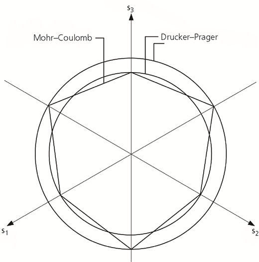
Comparison of Mohr–Coulomb and Drucker–Prager failure criteria in the deviatoric plane

In this model, the post-yield behaviour is described by the softening/hardening function Π(α_d) equal to (1 − βα_d)², where β is the softening/hardening parameter. This function fits well with experimental data, as demonstrated by Shao et al. (2003). The parameter β can be obtained from the post-yield stress–strain curve in triaxial tests; if the geomaterial softens, β > 0, and if it hardens, then β < 0.

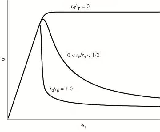
The parameters r_p and r_d are related by Equation 33 and govern the damage as shown in Figure 4. When r_d/r_p = 0, the model performs as a classical viscoplastic model and the damage mechanism is deactivated. However, when 0 < r_d/r_p ≤ 1·0, the model is allowed to undergo damage and therefore softening. The ratio r_d/r_p can be estimated by measuring the damage in the material. The variations of the elasticity modulus can be found in a displacement control triaxial test by carrying out a post-yield unloading/reloading cycle and comparing the values of the material stiffness with that of its original value before the yield stress is reached. There are other techniques for measuring damage in materials reported throughout the literature (see e.g. the paper by Lemaitre and Dufailly (1987)). If a rapid test is carried out and the damage α_d is plotted against the accumulative deviatoric plastic strain α_γ, then the ratio r_d/r_p can be estimated from the initial slope of the α_γ − α_d curve. From Equation 28

\frac{r_{p}}{r_{d}} \approx \sqrt{{(ρ \frac{d α_{d}}{d α_{γ}})}_{α_{d} \to 0}}

43

Figure 4

View large Download slide

Modelling coupled plasticity-damage behaviour

Two parameters are used to describe the viscoplasticity response; viscosity is defined by the parameter η, and the rate-sensitivity parameter is described by the non-dimensional parameter n. Both parameters are positive. These parameters are analogous to the parameters of the model by Perzyna (1966), which are widely used in computational applications of viscoplasticity and can be obtained using triaxial tests from the relationships given by Equation 30.

Numerical simulations and comparison with experimental data

The model has been specifically tested for its ability to reproduce a series of triaxial compression test results on three different geomaterials reported in the literature: (a) sandstone (Yang and Jiang, 2010), (b) Meuse–Haute/Marne claystone (Hu et al., 2014) and (c) Inada granite (Fujii et al., 1999).

Stress–strain response in drained triaxial tests

Yang and Jiang (2010) carried out drained triaxial tests on sandstone core samples extracted at the Xiangjiaba Hydropower Project in south-western China. The samples were taken at a depth of between 61·2 and 62·5 m, where the Poisson’s ratio and density are approximately ν = 0·22 and 2·600 Mg/m³, respectively. Triaxial loading tests under drained conditions performed on isotropically compressed samples were used to illustrate the short-term and the long-term behaviour.

The short-term loading tests were conducted under three different confining pressures (σ ₃ = 3, 5 and 7 MPa), and axial stresses were imposed at a constant rate of 0·127 MPa/s until peak strength was reached. The measured angle of friction φ was found to be about 58·4°. Table 3 shows the mechanical behaviour observed under triaxial compression. The peak axial strain ϵ _1p is defined as the strain value at rupture in terms of the complete stress–strain curve. The modulus of elasticity (E _s) refers to the slope of the approximately linear part of the stress–strain curve, while the modulus of deformation (E ₅₀) is defined as the slope between the original point and the stress at half-peak strength.

Table 3

Mechanical behaviours of sandstone samples under conventional triaxial compression (Yang and Jiang, 2010)

Confining pressure, σ ₃: MPa	3	5	7
Peak strength, (σ ₁ − σ ₃)_peak: MPa	163·6	180·7	209·6
Residual strength, (σ ₁ − σ ₃)_residual: MPa	43·0	42·2	44·7
Axial strain at peak strength, ϵ _1p: × 10⁻³	7·6250	7·6700	7·5556
Young’s modulus E _s: GPa	25·77	27·73	32·69
Young’s modulus E ₅₀: GPa	21·41	32·63	30·91

The parameters $c_{1}^{*}$ ⁠, $c_{2}^{*}$ and $c_{3}^{*}$ of the viscoplastic-damage model are calculated from the measured angle of friction φ and a dilatancy angle of φ/4 using Equation 42. Hoek and Brown (1997) studied the relationship between the angle of dilation ψ and the angle of friction φ and recommended that for a good-quality sample, ψ can be taken as φ/4. The average value of the Young’s modulus $(E_{50} + E_{s}) / 2$ for each sample is used in the numerical simulation (see Table 4). In the absence of the detailed testing procedure (described earlier) for obtaining the model parameters, the short-term loading test data for a confining pressure of 5 MPa are used to obtain the remaining model parameters. A Matlab software built-in standard Levenberg–Marquardt optimisation procedure has been utilised to estimate the set of material parameters. Table 4 shows the resulting set of material parameters used in the simulations.

Table 4

Viscoplastic-damage parameters used in the numerical simulation

Sample	$c_{1}^{*}$	$c_{2}^{*}$	$c_{3}^{*}$	η	n	r _p	β
Sandstone (Yang and Jiang, 2010)	21·95	1·83	0·55	5800	1·42	1·05	0·4
Claystone (Hu et al., 2014)	7·21	0·64	0·19	6000	3·00	1·08	0·5
Inada granite (Fujii et al., 1999)	31·39	1·86	0·56	6300	1·35	1·02	0·2

Sample	$c_{1}^{*}$	$c_{2}^{*}$	$c_{3}^{*}$	η	n	r _p	β
Sandstone (Yang and Jiang, 2010)	21·95	1·83	0·55	5800	1·42	1·05	0·4
Claystone (Hu et al., 2014)	7·21	0·64	0·19	6000	3·00	1·08	0·5
Inada granite (Fujii et al., 1999)	31·39	1·86	0·56	6300	1·35	1·02	0·2

Figure 5 shows the comparison between the short-term drained stress–strain response of the model and the experimental data with three different confining pressures. As can be seen from Figures 5(a)–5(c), the new coupled viscoplastic-damage model is remarkably successful in matching the general shape of the stress–strain response for all three confining pressures, at both peak stress and in the region of material softening.

Figure 5

View large Download slide

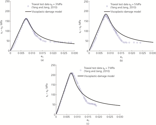
Comparison of model predictions and short-term stress–strain triaxial results for (a) σ ₃ = 3 MPa, (b) σ ₃ = 5 MPa and (c) σ ₃ = 7 MPa

Validation was also carried out with drained triaxial compression tests of saturated Meuse–Haute/Marne claystone. These tests were undertaken by Hu et al. (2014) on samples taken from a depth of about 521 m and were subjected to an in situ vertical stress of 12·7 MPa and horizontal stresses in the range 12·3–13·8 MPa. The axial strain rate in these tests was set at 10⁻⁷/s (corresponding to an average stress rate of 10⁻⁴ MPa/s). The measured angle of friction φ was found to be about 21·4°, and the cohesion c was found to be 3·94 MPa. The optimised parameters used in the analysis are shown in Table 3. Figure 6 shows the relationship between the radial strain and the axial strain at different confined pressures. This figure demonstrates that except for the case of high confining pressure (20 MPa), the new model can reasonably replicate the experimental data.

Figure 6

View large Download slide

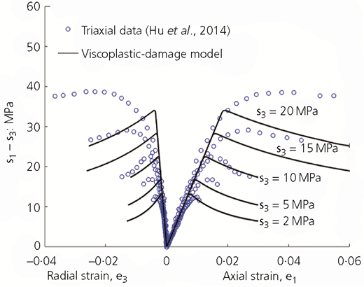
Comparison of model predictions and experimental results for drained triaxial with different confining pressures

Table 5 shows the evolution of the relative residual norm for a confining pressure of 5 MPa for three typical load increments. These results provide a clear indication of the good rates of convergence. The number of iterations needed to meet the convergence tolerance of ϵ _r = 10⁻⁸ is between three and four per load step.

Table 5

Return mapping residual norms for three typical load increments

Iteration	Increment 70	Increment 200	Increment 300
1	0·0354	0·2442	0·0575
2	1·65 × 10⁻⁴	0·0027	1·22 × 10⁻⁴
3	3·47 × 10⁻⁹	6·35 × 10⁻⁷	3·00 × 10⁻⁸
4	—	2·24 × 10⁻¹⁰	1·70 × 10⁻¹²

Strain–time response in creep triaxial tests

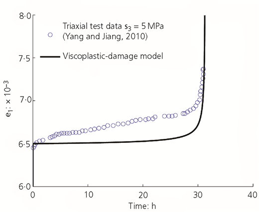
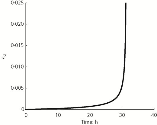
Yang and Jiang (2010) also conducted creep tests on sandstone in triaxial cells. In these tests, the deviator stress q = (σ ₁ − σ ₃) was kept constant. Figure 7 shows the comparison between the results of the viscoplastic-damage model and the experimental data for creep tests with a confined pressure of 5 MPa and a constant deviator stress of 160 MPa. The failure occurs after approximately 31·48 h. It can be seen that the general trend is well captured in terms of the time required to reach failure and the magnitude of axial strain. The evolution of the accumulative damage predicted by the model during the creep test is shown in Figure 8. It can be noticed that the accelerated damage rate follows a pattern similar to that of the accelerated creep strain. This is consistent with the experimental data of Heap et al. (2010), which show an accelerated rate of change in the pore volume of sandstone during tertiary creep.

Figure 7

View large Download slide

Model prediction: comparison with creep data (q = 160 MPa)

Figure 8

View large Download slide

Model prediction: evolution of damage with time

Validation is also made against triaxial creep tests on Inada granite reported by Fujii et al. (1999). These tests were conducted under a confining pressure of 10 MPa. The testing programme investigated the effect of creep stress on the strain–time behaviour. The numerical simulations were carried out with the parameters for Inada granite shown in Table 4. Figure 9 demonstrates that the viscoplastic damage model is capable of predicting the time required to failure at different stress levels.

Figure 9

View large Download slide

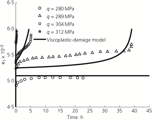
Comparison of model predictions and experimental results for triaxial creep tests (Fujii et al., 1999) at different deviatoric stresses

Limitations of the new viscoplastic damage model

Inherent or structural anisotropy is observed in many types of sedimentary rocks. The strength of the rock material strongly depends on the loading orientation with respect to the microstructure (Pietruszczak et al., 2002). The model presented here deals with isotropic damage only. Therefore, it is applicable only to the case of monotonic loading. The present formulation assumes that the dilatancy angle is constant and that there is a unique relationship between the plastic shear strain and the volumetric strain increments. Alejano and Alonso (2005) showed the dependency of the dilatancy angle on the confining stress and the material plasticity. The model is formulated in terms of triaxial stress space, and validation is carried out against triaxial data. It could be generalised by incorporating an appropriate Lode’s angle dependency function such as that suggested by Eekelen (1980). The strength parameters c ₁, c ₂ and c ₃ can be expressed as a function of Lode’s angle. However, further validation is needed. Furthermore, temperature dependency could be easily incorporated within the hyperplasticity approach as explained by Houlsby and Puzrin (2000).

Conclusions

In this paper, the authors have combined the continuum damage approach within the framework of hyperplasticity for rate-dependent materials, thus encompassing viscoplasticity and damage within a single theory. A novel coupled viscoplastic-damage constitutive model has been derived from two scalar potentials: a free-energy potential that provides the elasticity law and a dissipation potential that provides the yield function, the direction of plastic flow and the evolution of a damage variable. No additional assumptions are required. The model is formulated with few parameters that can be derived from conventional laboratory testing. It has been shown that the new model is capable of capturing the secondary and tertiary creep observed in soft rocks. Comparison with triaxial data has shown that the model provides a good approximation to short-term stress–strain curves obtained for different confining pressures and to long-term creep data.

Acknowledgement

The authors would like to thank the UK Engineering and Physical Sciences Research Council (EPSRC) for the PhD studentship awarded to the second author (Grant reference: EP/D504376/1).

REFERENCES

Al-Shamrani

MA

,

Sture

S

1998

A time-dependent bounding surface model for anisotropic cohesive soils

Soils and Foundations

38

61

-

76

A simple model for tertiary creep in geomaterials Open Access

Notation

Introduction

The hyperplasticity framework

Formulation of a new viscoplastic damage model

Integration of the constitutive model

Elastic predictor

Plastic correction

Consistent tangent operator

Selection of model parameters

Numerical simulations and comparison with experimental data

Stress–strain response in drained triaxial tests

Strain–time response in creep triaxial tests

Limitations of the new viscoplastic damage model

Conclusions

Acknowledgement

REFERENCES

Email Alerts

Suggested Reading

Related Chapters

Recommended for you

Cited By

Sharing Unavailable

A simple model for tertiary creep in geomaterials