
In this study, the dynamic response and instability of a low-permeability deformable caisson-type quay wall (CQW) with backfill soil exposed to standing waves is evaluated. The focus is on the dynamic response and instantaneous liquefaction of seabed and backfill around the CQW. This study aims at closing the knowledge gap about the wave-induced CQW–seabed response without the presence of a breakwater, as the bulk of the prior research has been done on CQWs considering earthquakes as the primary loading source. Finite elements are used, and numerical results are obtained in terms of displacements, pore-pressure and shear stress variations in temporal and spatial domains. Wave-induced instantaneous liquefaction is analysed, and analyses are performed to determine the effect of soil/wave properties on dynamic response and liquefaction. Results indicate that there is considerable liquefaction potential in both seabed and backfill that may play a key role in the stability of the CQW. While such a response is dependent upon the induced wave energy and the CQW motion, seabed parameters alter the instantaneous liquefaction occurrence as well. A slight decrease in the seabed degree of saturation causes a contraction behaviour under the wave-induced motion of the CQW, which, in turn, affects the mechanism of response and the initiation of instability in the seabed.
Notation
- Bp
strain–displacement matrix for pressure
- Bu
strain–displacement matrix for displacement
- C
damping matrix of total system
- Cf
damping matrix of pore fluid
- Dijkl
tangent constitutive matrix
- d
water depth
- E
elasticity modulus
- gi
acceleration of gravity
- H
wave height
- K0
earth pressure coefficient
- Kf
pore water bulk modulus
- Kf
stiffness matrix of pore fluid
- Kp
bulk modulus of the fluid
- Ks
stiffness matrix of solid
- k
wave number
- ki
permeability tensor
- ks
seabed permeability
- L
wavelength
- Ms
mass matrix of solid
- Msf
mass matrix of pore fluid
- m
Kronecker delta vector
- Np
shape function matrix for pore pressure
- Nu
shape function matrix for displacement
- n
porosity
- p0
absolute pressure
- p
pore pressure
- q0
wave amplitude
- qi,j
wave pressure
- Sm
total effective mean stress
- T
wave period
- t
time
- u
solid displacement
- ν
Poisson’s ratio
relative fluid displacement
- x
Cartesian horizontal coordinate
- z
Cartesian vertical coordinate
- γ
unit weight
- γw
unit weight of water
initial strain
- ρf
fluid density
- ρ
total density
- σij
stress tensor
- τs
shear stress
- τf
shear strength
- ω
wave frequency
Introduction
The wave-induced hydro-mechanical response of saturated porous seabed is an important problem in coastal and offshore geotechnics. In relation to that, dynamic response is analysed based upon the key wave characteristics and physical properties of seabed used to decide feasible formulations for a particular soil–offshore structure system. Quay walls are one such structural system; they constitute a part of marine infrastructure built to protect ports and harbours. They are one of the most common types of such sets built as they are both durable and capable of reaching deeper soils while at the same time being easy to construct. Caisson-type gravity quay walls (CQWs) are frequently used to serve such a purpose; they are proven to withstand both cyclic and breaking wave loads. While the main goal of building such structures is to maintain stable coastlines against severe seismic and ocean wave action, they also act as a solid barrier for the structures on and around the shore surface. Therefore, quay walls are typically built as a common component of a port system to sustain integrity. Three main criteria have generally been considered in the design of gravity quay walls – namely, sliding, overturning and bearing capacity of the foundation (Alyami et al., 2007; Dakoulas and Gazetas, 2005; Iai et al., 1998). Until now, plenty of studies have focused on satisfying such criteria under monotonic and cyclic loads. Also, the majority of the studies investigating the response of CQWs mostly examine the seismic-induced dynamic response of CQWs since there is generally some kind of a breakwater structure temporarily or permanently protecting their construction against ocean waves (Alyami et al., 2007; Dakoulas & Gazetas, 2005; Iai et al., 1998; Iai and Sugano, 2000; Ichii et al., 2000; Inagaki et al., 1996; Inoue et al., 2003; Nozu et al., 2004; Sugano et al., 1996). That being said, there are cases where the quay walls should withstand severe wave forces without the presence of any breakwater structure at the port, which puts coastlines and industrial and residential establishments at great risk (i.e. the Ambarlı Port in Istanbul and the Asya Port in Tekirdağ, Turkey). In such cases, quay walls are exposed to major wave forces, posing a threat for the stability of the port. Therefore, there is an important gap in the state-of-the-art knowledge requiring theoretical and numerical studies for understanding the CQW response. Wave-induced liquefaction becomes the leading phenomenon governing the stability of quay walls; however, this issue has not really been investigated for CQWs before.
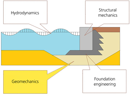
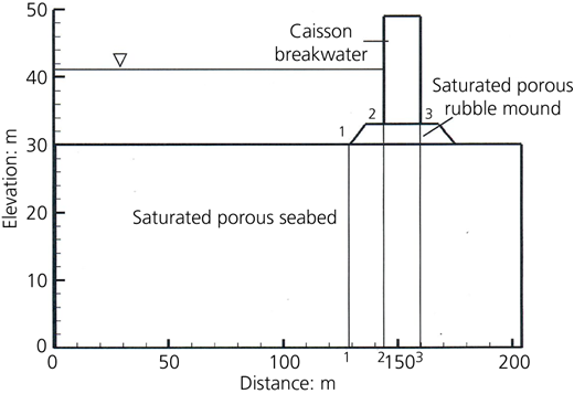
The problem is multi-disciplinary since it involves many fields brought together for understanding the actual dynamic response of the fluid–soil–structure system (Figure 1) in terms of the seabed stability, structural stability and wave mechanism. Many studies conducted over the last few decades on seabed-foundation behaviour make use of geomechanics for a true coverage of the dynamic soil response. The theory of poroelasticity, developed first as the theory of consolidation by Terzaghi (1925) for a one-dimensions soil, plays a major role in modelling the actual response. Then, Biot (1941) generalised the theory to three dimensions and subsequently included the dynamic terms (Biot 1955, 1962) essentially to develop a complete theory of coupled flow and deformation. Detournay and Cheng (1993) summarise the constitutive equations necessary to combine with the Biot formulation. Among many other previous studies in coastal and offshore geotechnics, works by Okusa (1985), Goda (1985), Lundgren et al. (1989), Zen and Yamazaki (1990), Hsu and Jeng (1994) and Rahman et al. (1994) are some of the pioneering studies investigating the effect of seabed response. Another study includes the analysis of pore pressure and effective stress in coastal structures (Mase et al., 1994). In addition to analytical solutions, numerical models have been developed for the dynamic response and liquefaction around marine structures (Zienkiewicz et al., 1999).
The stability of seabed underneath marine gravity structures subjected to wave loads is studied by De Groot et al. (2006) and Kudella et al. (2006), who conducted large-scale model experiments to investigate the instantaneous and residual pore pressure generation under a caisson breakwater. In the paper by Jeng and Seymour (2007), two mechanisms for seabed liquefaction are shown by a specific condition. Most of such work on the oscillatory mechanism for liquefaction is reviewed by Jeng (2003). Zen and Yamazaki (1990) address the role of instantaneous liquefaction on marine sediments. Mory et al. (2007) present the field data for liquefaction. Other noteworthy studies on the instantaneous liquefaction include those of Sakai et al. (1992, 1995), Nago et al. (1993), Sumer et al. (1999); Choudhury et al. (2006); Dunn et al. (2006); Ulker (2012); Ulker et al. (2012) and Kirca et al. (2014).
Standing wave effects have been investigated for caisson-type structures (Kudella et al., 2006; Tsai and Lee, 1995; Ulker et al., 2010). Some study results show that the residual liquefaction causes the structural blocks to sink in such a liquefied soil as a result of self-weight (Sumer et al., 1999; Suzuki et al., 1998). The major cause of the sinking of breakwaters has been investigated in terms of instantaneous liquefaction (Sakai et al., 1995; Sumer and Fredsøe, 2002; Ulker, 2012; Ulker et al., 2010, 2012). Recently, the effect of the degree of saturation on the instantaneous liquefaction of seabed around a rubble mound breakwater has been presented by Ulker et al. (2018). Another important aspect for multi-component coastal–offshore systems is the condition where there is a non-homogeneous seabed involving multiple soil types interacting with one another or a single soil with heterogeneous properties (Zhang et al., 2016). In relation to this study, the dynamic response and instability of a CQW–seabed system located at the port of Kobe, Japan, which was damaged during the Hyogo-Ken Nanbu earthquake, has been investigated (Baksı, 2017).
The objective of this study is to understand the wave-induced dynamic response of a CQW and the conditions leading to the instability of the system under standing waves. The motivation is that the wave-induced CQW–seabed response without a breakwater in the vicinity is not fully known, as the bulk of the prior research has been done on quay walls considering earthquakes as the primary source of excitation. Hence, a low-hydraulic-conductivity and deformable CQW under waves is investigated. Standing wave-induced pore pressures, soil displacements and stresses are evaluated, and the instantaneous liquefaction potential of a CQW–rubble–seabed system is investigated using finite elements (FEs).
Dynamic response of seabed
Governing equations
The governing equations for the dynamics of saturated porous seabed were developed by Biot (1941, 1955, 1962), considering the balance principles of the solid and fluid phases (i.e. pore water). The flow is governed by Darcy’s law, which is included in the equilibrium equations. The equation system is written as
where the first term of Equation 1 is the total stress divergence, the second one is the body force and the other terms are the inertias linked with relative pore water displacement () and the displacement of the solid skeleton (), respectively. The terms of Equation 2 are the gradient of the pore pressure (p), the fluid body force and the drag term of Darcy’s law, with the last two terms being the inertias. Also, k i and n are the permeability tensor and porosity, respectively. Equation 3 has the volumetric strain term of the solid part as well as the rate of volumetric strain of pore water and the rate of change of pore pressure. Here, K f is the pore water bulk modulus and, along with the degree of saturation, is used in getting the compressibility of pore water through
where p 0 is the absolute pressure and K p is the bulk modulus of the fluid. The strain–displacement relation, along with the stress–strain relationship, completes the formulation:
where is the tangent constitutive matrix and is initial strain. Eliminating the inertial terms associated with pore water yields the so-called partially dynamic (PD) formulation, which is written in the form
and further eliminating solid motion accelerations results in the quasi-static (QS) form.
Finite-element formulation
The FE model is developed by discretising the above equations over the spatial domain. The equation below is the matrix form of the final equation of motion as a result of the PD formulation (Equations 8–10) as
where
, , , , , and , ,
Here, m is the Kronecker delta vector, K s and K f are the stiffness matrices of solid and pore fluid phases, C and C f are the damping matrices of the whole system and the pore fluid, M s and M sf are the mass matrices of solid and pore fluid, B p and B u are the strain–displacement matrices for pressure and displacement, and N p and N u are the shape functions of pore pressure and the displacement. Eight-node quadrilateral interpolation functions are utilised for the quadratic approximation of the displacement degree of freedom, and four-noded bilinear shape functions are defined for the approximations of pressure to satisfy spatial convergence. Isoparametric element formulation is utilised to handle the spatial integration accounting for element distortions. The above formulation, as well as the QS form derived neglecting the mass matrix given below
are implemented in a computer program. Equation 11 can be written in a single form:
where u and p in the degree of freedom (DOF) vector X are the only field variables and ‘n + 1’ is the time step number.
Verification analyses
In this section, a number of analytical and numerical solutions for the above formulations of the dynamic response of porous media under various loadings are developed to solve boundary value problems associated with seabed dynamics. The results are then verified with available solutions from the field.
In the first problem, the wave-induced dynamic seabed response under a linear progressive wave in free field (Figure 2) is studied. Results are presented in terms of the distributions of shear and effective stresses as well as pore pressure with depth for various values of wave and seabed parameters. The verification of numerical solutions is given in Figure 3 using the analytical solutions of Ulker and Rahman (2009). Results are normalised with respect to wave magnitude
where k is the wave number, d is the water depth and H is the wave height.
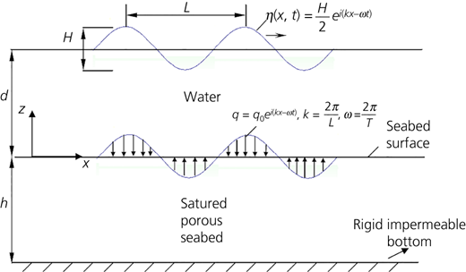
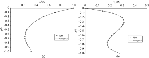
PD formulation: (a) pore pressure, (b) shear stress response; T = 1 s, L = 20 m, h = 10 m, k s = 0.001 m/s
PD formulation: (a) pore pressure, (b) shear stress response; T = 1 s, L = 20 m, h = 10 m, k s = 0.001 m/s
In the second problem, the wave-induced response in front of a vertical wall is evaluated. The paper by Tsai and Lee (1995), which provides the analytical solutions and experimental results for the standing wave-induced seabed response in front of a vertical wall in terms of pore-pressure distributions for a wave period of T = 1 s, is used to verify the results, which match fairly well (Figure 4).
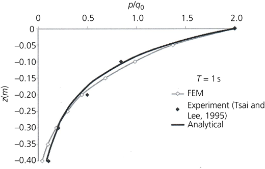
Comparison of standing wave-induced pore pressure response in front of a caisson breakwater for T = 1 s (k s = 1.2 × 10⁻⁶ m/s, H = 5.1 cm, S = 0.98). FEM, finite-element method used to obtain the solution
Comparison of standing wave-induced pore pressure response in front of a caisson breakwater for T = 1 s (k s = 1.2 × 10⁻⁶ m/s, H = 5.1 cm, S = 0.98). FEM, finite-element method used to obtain the solution
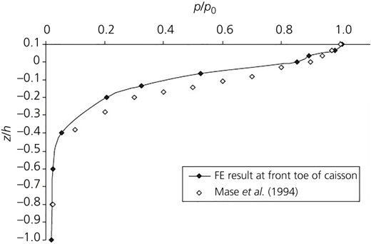
The last verification is performed on a breakwater problem given in Figure 5. In the problem, a caisson breakwater built on a granular seabed is exposed to standing waves using the FE formulation presented in this study. Figure 6 presents the response results of seabed at the breakwater front face in comparison with those of Mase et al. (1994).
Analysis of caisson-type quay wall–seabed problem
In this study, a CQW with a rubble foundation and backfill soil is studied in terms of wave-induced response. The quay wall examined is the one that failed during the Kobe earthquake at the Kobe port. The entire soil–structure system is analysed using the classical FE method, and the response of the CQW–soil is computed in terms of displacements and pore pressures as well as effective and shear stresses in the seabed around the CQW.
Caisson-type quay wall model
In this section, a plane-strain FE model is built using the structural and material properties based on the actual cross-sections of the CQW at the Kobe port (Figure 7). The material zones are: (a) saturated backfill, (b) seabed soil, (c) rubble mound, (d) clay layers and (e) caisson quay wall. As far as the boundary conditions, on the left seabed lateral boundary, time-dependent variations of DOF for the analytical solutions obtained for a single layer in free field are prescribed.
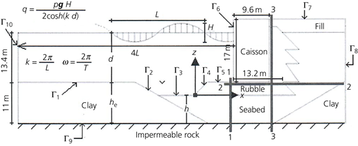
The reason for this is, the further away from the caisson, the more dominant the free-field seabed response gets under progressive waves, and the effect of the structure will recede. Thus, the left lateral boundary is accurately located at such a place, and its physical effects are neglected in terms of the numerical values of DOF and stresses on the dynamic response of the CQW. Therefore, the minimum distance required to have such an effect without a significant change in response around the CQW is determined to be about four times the incoming wavelength. It should be noted here that convergence checks of related FE analyses in spatial and temporal domains are carried out and the optimum mesh has been used in the subsequent parametric analyses.
As for other boundary conditions, the bottom boundary is considered impermeable and constrained for vertical and horizontal displacements. Also, the right lateral boundary is assumed to be located far enough away not to influence the dynamic response of the CQW. Horizontal displacement and pore pressure are assumed to vanish along the right side. Lastly, along the surfaces of seabed and at the front face of the caisson, simple standing wave-induced pressure in the form given below is applied:
where q i,j is the wave pressure, q 0 is the wave amplitude, k is the wave number and ω is the wave frequency. All the boundary conditions are presented in Table 1. Here, a more sophisticated wave form with higher-order wave terms could also be used to calculate the wave pressures acting on the CQW, accounting for the effect of trench height on the wave form; however, the present research focuses more on identifying the simplest mechanism controlling the response around the quay wall in this study.
Boundary conditions of CTQ-seabed system
| Boundary number | Condition |
|---|---|
| Г1−Г6 | p = [(ρgH/2)cosh(kd)]cosh(kz)cos(kx)cos(ωt) |
| Г7 | p = 0 |
| Г8 | ux = uz = p = 0 |
| Г9 | ux = uz = dp/dn = 0 |
| Г10 | Obtained from the free-field analytical solution |
It should also be noted that in this study, the concrete caisson quay wall is considered as a massive structure, hence it being the ‘gravity type’. Thus, it is plausible that one neglects the relative movement of the massive quay wall and the surrounding rubble under wave loads with wave periods that do not trigger large relative deformations. Also, the quay wall is considered to have a rough concrete surface, allowing compliant motion with respect to the backfill and seabed soils around. The results in terms of variable distributions are obtained for sections 1–1, 2–2 and 3–3, as shown in Figure 7. In the next section, the results of a number of parametric studies considering key wave and soil parameters such as permeability and wave period are presented. Table 2 shows the values of parameters used in the analyses.
Numerical values of the parameters used in CQW-seabed analyses
| Properties | Symbol | Value: unit |
|---|---|---|
| Seabed density* | γ S | 1.75, 1.72, 2.07: t/m3 |
| Seabed Young’s modulus* | E S | 16, 20–40, 260: MPa |
| Seabed Poisson’s ratio* | v S | 0.33, 0.33, 0.30 |
| Seabed permeability | k S | 10−6 – 10−4 – 10−2: m/s |
| Seabed porosity | n S | 0.28–0.35 |
| Seabed saturation | S S | 1.0 |
| Clay density | γ C | 1.7: t/m3 |
| Clay Young’s modulus | E C | 10 330: kPa |
| Clay Poisson’s ratio | v C | 0.4 |
| Clay permeability | k C | 10−8: m/s |
| Clay porosity | n C | 0.5 |
| Clay saturation | S C | 1.0 |
| Rubble density | γ R | 2.00: t/m3 |
| Rubble Young’s modulus | E R | 160 000: kPa |
| Rubble Poisson’s ratio | v R | 0.33 |
| Rubble permeability | k R | 0.1: m/s |
| Rubble porosity | n R | 0.25 |
| Rubble saturation | S R | 1.0 |
| Caisson density | γ W | 2.5: t/m3 |
| Caisson Young’s modulus | E W | 2 × 10⁷: kPa |
| Caisson Poisson’s ratio | v W | 0.18 |
| Water depth | d | 13.4 (m) |
| Wave length | L | 38–104–165: m |
| Wave height | H | 1.15–3.1–5.58: m |
| Wave period | T | 5–10–15: s |
*Values correspond to GM-SP-GW soils, respectively
Dynamic response of the system of caisson-type quay wall
In this section, the effect of permeability (k s), wave period (T) and seabed soil type are considered in the parametric studies. The responses are obtained in terms of the distributions of absolute value vertical displacement, pore pressure and shear stress along three cross-sections. Pore pressure and stresses are normalised with respect to the wave amplitude q 0 = ρ w gH at section 1–1. Lateral x-distance is normalised with total section lateral distance (X 0) at 2–2. It is also taken into account that the variation in wave period values changes the wavelengths according to the dispersion formula in the linear wave theory as
where g is acceleration of gravity and L is the wavelength (Dean and Dalrymple, 1991).
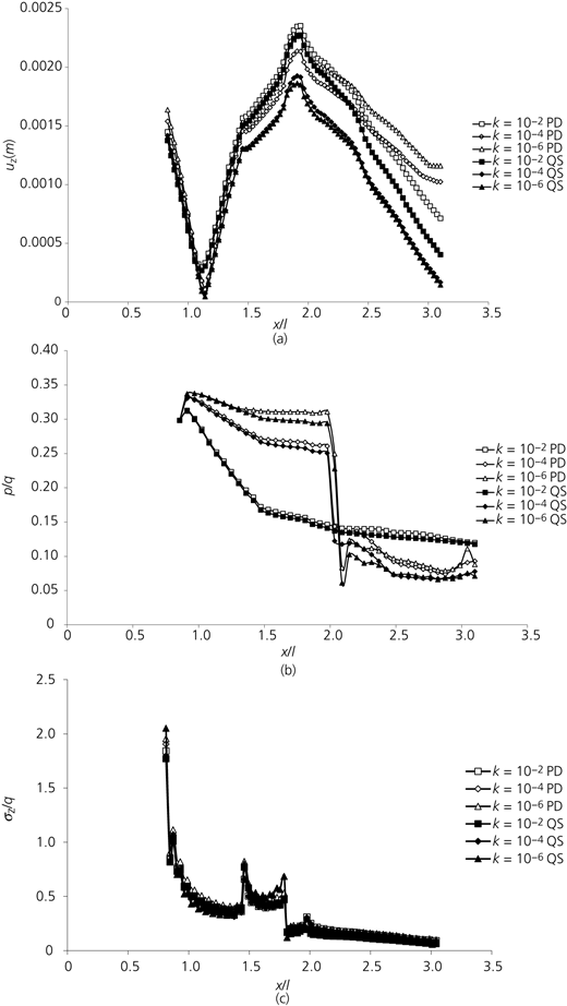
Effect of seabed permeability
When it comes to seabed and its properties, one of the first governing quantities is permeability. In the construction of CQWs, soils closer to the seabed surface are typically filled with coarser-grained stiff materials that work as stable soils sustaining their bearing capacity during the wave-induced cyclic shearing process. It is desirable that seabed material should possess a permeability value in a range such that there will not be a hydraulic gradient large enough to create a seepage force that overcomes the overburden pressure of the seabed. In that case, the hydraulic gradient reaches a ‘critical value’, triggering a condition occurring due to a process called instantaneous liquefaction.
When the response along section 1–1 is examined, it can be seen that dynamic response is clearly a function of seabed permeability. However, as the permeability decreases, there is an increase in the displacements in both directions. The system also gives the same response in PD solutions; however, the result is that the increase in displacements becomes more obvious (Figure 8(a)). As the permeability difference between seabed and rubble mound decreases, pore pressures get closer to each other for section 1–1 (Figure 8(b)). Especially for the seabed with k = 10−2 m/s, the distribution of pore pressures is rather uniform. In regard to this, the effect of a small difference in permeability between rubble and seabed cannot be discarded. Moreover, it should be noted that inertial terms are at negligible levels. With the decrease in permeability, the effect of inertial terms becomes apparent, as well as the pressure differences between seabed and rubble mound. Due to caisson rocking motion, shear stress accumulation occurs at the toes (Figure 8(c)).
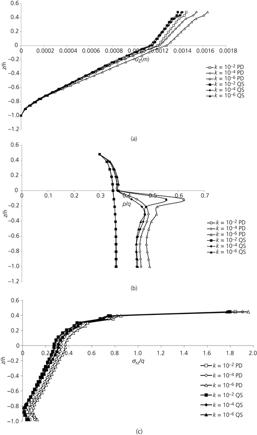
Effect of permeability on (a) displacement, (b) pore pressure and (c) shear response in 1–1
Effect of permeability on (a) displacement, (b) pore pressure and (c) shear response in 1–1
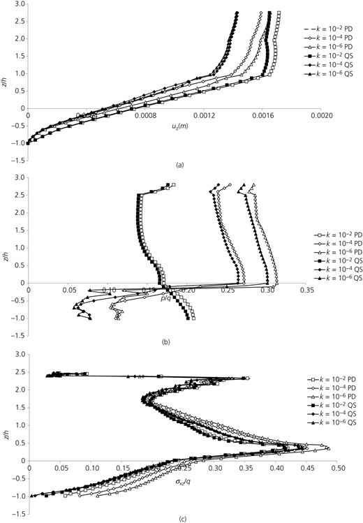
Figure 9 shows the results along section 2–2. Vertical displacements are particularly large at the toe of the caisson wall due to the rocking (Figure 9(a)). Away from the wall, the effects of the change in permeability values on the vertical displacements become more apparent. The largest displacement occurs in between the rubble backfill and seabed.
Effect of permeability on (a) displacement, (b) pore pressure and (c) shear response in 2–2
Effect of permeability on (a) displacement, (b) pore pressure and (c) shear response in 2–2
It is observed that there is a gradual decrease in pore pressure in the rubble under the caisson (Figure 9(b)), which is directly associated with the large permeability of the rubble. In general, the increase in permeability values results in a pore pressure decrease. Also, for this region, the dynamic effects become apparent when inertial terms are introduced. At the rubble–seabed interface, the difference in pore pressures increases due to the discontinuity in permeability. The sudden and large decline of pore pressures at the back toe of the caisson may be explained by an occurrence of possible piping behaviour for k = 10−4–10−6 m/s, which poses an important and common problem in offshore geotechnical engineering. Along section 2–2, shear stresses gradually decrease in the seabed (Figure 9(c)), while showing the shearing of the caisson–seabed interface. This is subsequently studied further.
Figure 10(a) shows the vertical displacements in the seabed in section 3–3. Dynamic effects are noticeable with the largest effect being for k = 10−4–10−6 m/s. Figure 10(b) shows the variation of pore pressures. When the permeability difference between seabed and the rubble increases, pore pressure variations and the effect of inertial terms also increases, except for the shear (Figure 10(c)).
Effect of permeability on (a) displacement, (b) pore pressure and (c) shear response in 3–3
Effect of permeability on (a) displacement, (b) pore pressure and (c) shear response in 3–3
Effect of seabed soil type
The types of soils that are common in coastal environments are typically granular soils such as sand. Occasionally, it is known that there are clayey sand layers or that there is some thin clay layer overlying a granular medium (Soltanpour et al., 2010; Ulker, 2012). Some other granular soil types can also be present in the seabed and also be used as a fill material behind quay walls (Alyami et al., 2007). The details of the authors’ analyses are based on the actual properties of the Port Island soils located in Kobe, Japan whose seismic response was investigated previously against the Hyogoken-Nanbu earthquake (Alyami et al. 2007; Dakoulas and Gazetas, 2005; Iai et al., 1998). The properties of the materials have been determined initially from those studies. Then, considering all the material properties, the most suitable group symbol is determined for those soil layers to make it easier to identify and distinguish different seabed soils in presenting the results and highlight the effect of such soil types. Regardless of the group symbols, particle size characteristics are not specifically considered.
In this section, various graded mixtures are used as seabed soil material; a silty sand–gravel mixture (GM), a poorly graded medium dense sand (SP) and a well-graded sand–gravel mixture (GW) are chosen. It should be noted that such soil types are less indicative of their symbols but more distinctive in terms of the elasticity modulus, E, Poisson’s ratio, ν, permeability and unit weight, γ. That is, the representative parameter in the dynamic analyses of the seabed–CQW system in this section is, in fact, the rigidity of the seabed soil.
Results show that the effect of inertial terms in the PD solution becomes more pronounced in displacements with the change in soil types. In section 1–1, low differences occur in the response of PD and QS solutions for GW soils, which might be due to the permeability of the medium. For SP and GM soils, inertial terms play an effective role on the displacements (Figure 11). The changes in pore pressure normalised by standing wave amplitude are compared for different soil types in section 1–1. In view of this, a change in soil types does not lead to a significant difference in the rubble mound. So, even if the soil in the lower layer varies, the upper rubble layer is not affected much as far as pore pressure differences are concerned. It should also be noted here that for the rest of the figures in this section, it is sufficient to present only the degree for freedom response and leave out the stress variations.
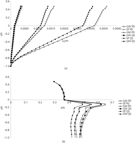
Effect of soil type on (a) vertical displacement and (b) pore pressure in section 1–1
Effect of soil type on (a) vertical displacement and (b) pore pressure in section 1–1
In section 2–2, in the case of SP soil, dynamic effects are noticeable (Figure 12) and displacements increase as compared to GW. For a GM-type soil, displacements increase further and reach a maximum when combined with the dynamic effects, particularly at the intersection of rubble and backfill. As shown in Figure 12(b), pore pressures are slightly higher in the SP soil, but past the rubble zone, all pore pressures display a sudden decrease, which might be attributed to void redistributions in the rubble essentially playing an increasing role in the permeability of the rubble compared to seabed. Although it is not quite possible to exactly model such micro-level behaviours with the current continuum formulation, such alterations may surface their macro-level effects at certain locations in the model. Within the seabed, dynamic effects are also more pronounced.
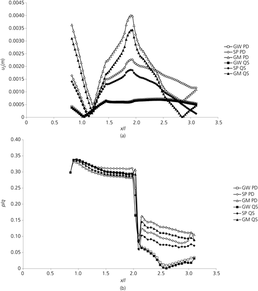
Effect of soil type on (a) displacement and (b) pore pressure in section 2–2. GM, silty gravel; GW, well graded gravel; SP, poorly graded sand
Effect of soil type on (a) displacement and (b) pore pressure in section 2–2. GM, silty gravel; GW, well graded gravel; SP, poorly graded sand
Effect of wave period
Figure 13 presents the results for different wave periods. Inertial terms are increasingly influential on the dynamic response of the seabed. In the rubble, the inertial terms associated with the solid phase in the seabed do not affect the rubble motion. As the wave periods decrease, a respective increase in pore pressures is observed in the seabed. The possibility of getting closer to the natural period of the CQW–seabed system resulting in T = 10 s analyses may be considered, which reveals such an intermediate response. The peak values of reactions occur between certain period values. For example, the dynamic effects observed for T = 10 s are in between those observed for 5−15 s (Figures 13(a) and 13(b)).
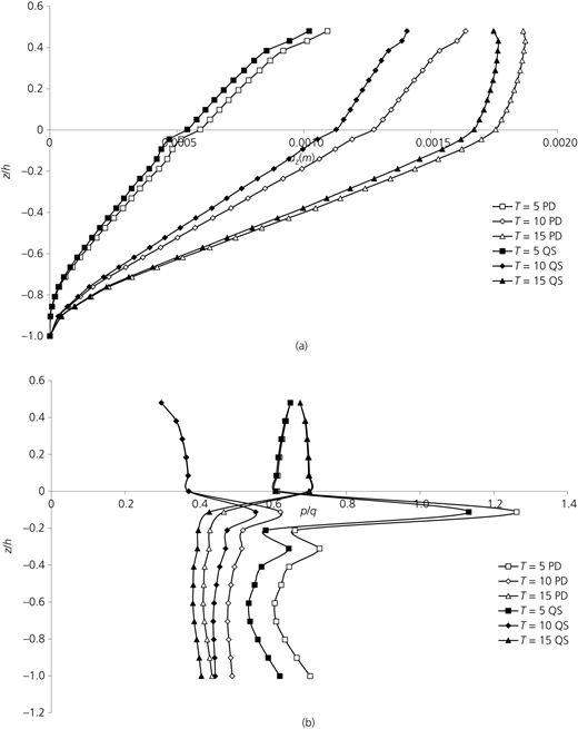
Effect of wave period on (a) vertical displacement and (b) pore pressure in section 1–1
Effect of wave period on (a) vertical displacement and (b) pore pressure in section 1–1
Figure 14 shows that the increase in periods makes it possible to observe the dynamic effects on the response of the system. In particular, displacements for 10 s and 15 s in the seabed are close to one another. It is interesting to note that displacements increase again after a certain point. This shows that more damage can occur in the interior part of the harbour, which is essential to know prior to any design of such a CQW. In this particular case, for k = 10−6 m/s, settlements are larger for the outlier 10 s period in the PD analysis. On the lower part of the CQW and in the rubble, a large difference between the pore pressures is obtained at section 2–2 in Figure 14(b). In particular, the values obtained for T = 10s are considerably lower than others, which shows that the large values for different specific standing wave periods can occur in a dynamic analysis.
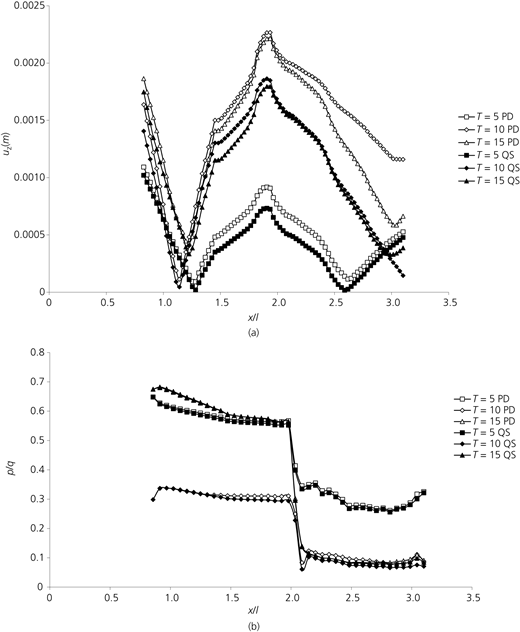
Effect of wave period on (a) vertical displacement and (b) pore pressure in section 2–2
Effect of wave period on (a) vertical displacement and (b) pore pressure in section 2–2
The variation of vertical displacements with wave periods gives interesting results in section 3–3 (Figure 15(a)). According to the results obtained from the PD formulation, minimum displacements are obtained for 5 s, and there is a noticeable increase in the values when the effect of dynamic terms is taken into consideration. On the other hand, the displacements obtained in the QS solution, especially for 10 s and 15 s, are higher in the rubble layer than they are in the PD solution.
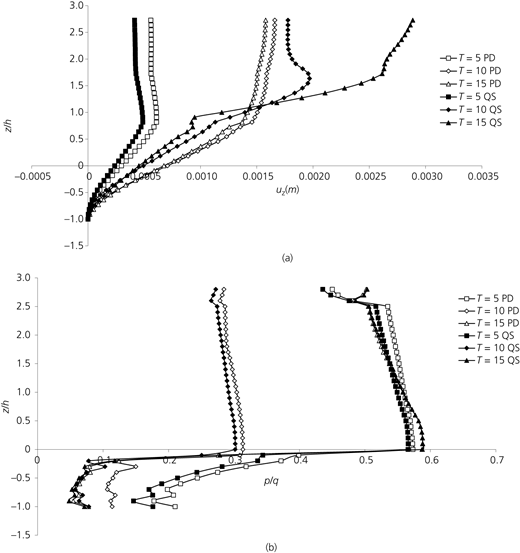
Effect of wave period on (a) vertical displacement and (b) pore pressure in section 3–3
Effect of wave period on (a) vertical displacement and (b) pore pressure in section 3–3
Instantaneous liquefaction in caisson-type quay wall–backfill–seabed system
Just like for other coastal structures, CQWs are under the constant attack of wave loads. This effect not only changes the physical conditions (displacements, strains etc.) of the underlying soil layers, but it also adversely affects the structural stability conditions. The reason for this is that marine soils are susceptible to wave-induced liquefaction, resulting in failure of coastal structures through their foundations. Liquefaction is an important phenomenon that occurs practically in two ways: one being generated in saturated loose sandy soils where effective stress vanishes due to the gradual build-up of pore pressure under wave action and the other occurring typically in slightly unsaturated sediments under tensile wave forces as a result of overcoming effective in situ mean stress due to induced upward seepage force (Figure 16).
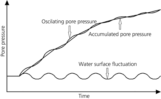
The former is called residual liquefaction, while the latter is generally termed as instantaneous liquefaction. In either case, soil as a whole acts like a fluid flowing without exhibiting any shear strength, either instantaneously or from that moment on during wave action. Once liquefaction occurs, the structures resting on the liquefied seabed sink. In this study, the wave-induced instantaneous liquefaction is investigated around the CQW. Firstly, to validate the numerical methodology used to calculate the depth of liquefaction, the results of the free-field seabed problem under standing waves in front of a vertical wall are compared with that of Tsai (1995). This study provides a basis for the subsequent analyses of the system. Here, the liquefaction prediction criterion based on the mean effective normal stress given below is used:
Here, the first term is the in situ mean effective stress and the second is the mean effective stress induced by the wave. Tension is taken as positive, and K0 is the earth pressure coefficient at rest. Figure 17 shows the maximum liquefied area obtained at a specific time step during a free-field FE analysis conducted with the presented numerical model.
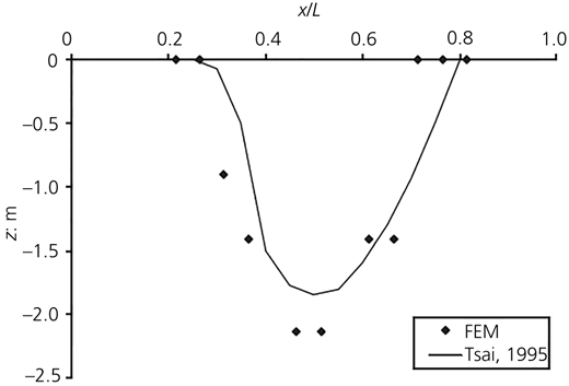
Comparison of liquefaction depths in free field between Tsai (1995) and this study (FEM) (T = 8 s, L = 70 m, hs = 10 m, H = 4.2 m, h = 30 m, Kf = 10 MPa)
Comparison of liquefaction depths in free field between Tsai (1995) and this study (FEM) (T = 8 s, L = 70 m, hs = 10 m, H = 4.2 m, h = 30 m, Kf = 10 MPa)
Carrying on with this numerical formulation, in this section, instantaneous liquefaction potential is studied around the CQW–seabed–backfill system with a number of parametric studies. In the analyses, the following mean effective stress criterion is used (Ulker et al., 2012, 2018):
which also includes the term associated with effective-stress increase due to the CQW weight.
Numerical modelling of liquefaction
In this study, the analysis of instantaneous liquefaction is evaluated in three phases. This has been applied before by the first author and various co-authors (Ulker et al., 2010, 2012, 2018). Firstly, a free-field seabed layer with the same properties as the ones in the CQW model is loaded with hydrostatic progressive wave pressure, including the body forces essential to model the consolidation phase. Secondly, the response of the seabed (both for QS and PD) along the lateral boundaries of the free field in terms of displacement and pore pressure DOF are recorded. Then, the actual CQW–seabed model is developed where the free-field DOF response time histories are applied as single-point constraints along the left lateral boundary, which is allowed to consolidate under the hydrostatic force of the ocean water as well as self-weights. Such an analysis yields settlements and effective stresses at the end of consolidation, which are then introduced into the third phase of the analysis as the initial conditions to simulate standing wave-induced instantaneous liquefaction. The standing wave pressure, p, is calculated as
in which γ w is the unit weight of water. Once again, more sophisticated wave forms with higher-order terms can be applied here; however, such a complexity is out of the scope of this study. This three-phase analysis procedure mimics the actual field stress and pore pressure conditions leading to liquefaction more accurately. In the FE analyses of instantaneous liquefaction, the total effective mean stress (S m) in Equation 17 is calculated in the soil. Here the depth of liquefaction is identified at respective lengths of time.
Effect of seabed permeability
The instantaneous liquefaction of seabed is directly affected by the seabed permeability (Figure 18). That is, the rocking motion of the wall causes a change in variation of internal stresses and development of pore pressures in the backfill, which is controlled to a large extent by the soil permeability. For large values of permeability (k s = 10−2 m/s), there is a large amount of water flow in the upward direction in the backfill, triggering liquefaction. A similar response is obtained for k s = 10−4 and 10−6 m/s in the backfill; however, the amount of liquefaction in seabed is less than it is for k s = 10−2 m/s, which occurs along the left interface between seabed and the clay slope. There is also a considerable amount of liquefaction at the slope corners regardless of the seabed permeability due to large wave forces.
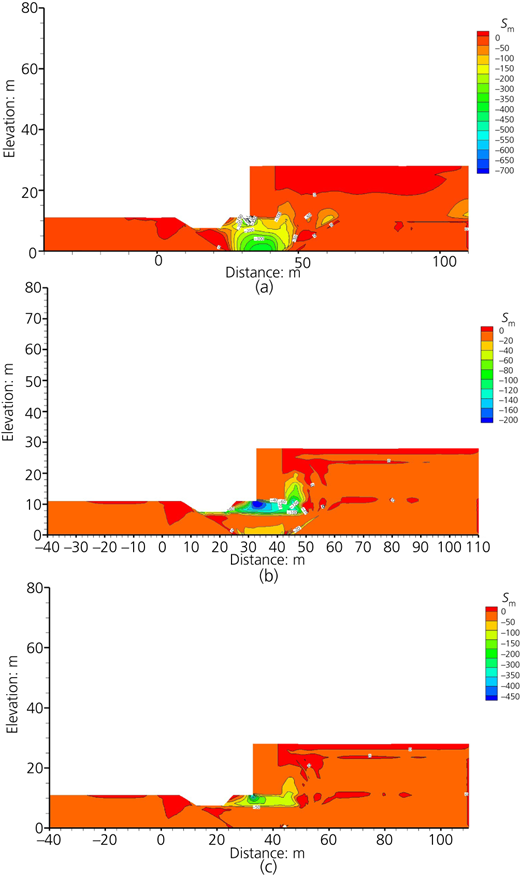
S m variation for SP, Ss = 0.99, T = 10 s, k s (m/s) (a) 10−2, (b) 10−4, (c) 10−6, PD (in kPa)
S m variation for SP, Ss = 0.99, T = 10 s, k s (m/s) (a) 10−2, (b) 10−4, (c) 10−6, PD (in kPa)
Effect of inertial terms
Figures 19 and 20 show the effect of inertial terms on the instantaneous liquefaction. For T = 10 s and for two permeability values, there is slight difference in the seabed and rubble between the QS and PD results, while there is considerable discrepancy in the liquefaction response in the backfill. The PD solution is negatively discriminated in liquefied regions for 10 s waves. Another noteworthy point is that the CQW backfill exhibits tensile mean stress, causing localised liquefaction due to the motion of the quay wall. This becomes apparent for k s = 10−4 m/s and E = 20 MPa analysis as in Figure 20, where the QS formulation yields slightly larger areas. Though that is the case, the PD solution for k s = 10−4 m/s results in more liquefaction both in the seabed and in the clay surface, which is basically the more conservative result. Relatively slower flow through the porous soil for the 10 s–10−4 m/s combination (Figure 20) responds to the wave action in such a way that the QS result seems to capture the behaviour rather well.
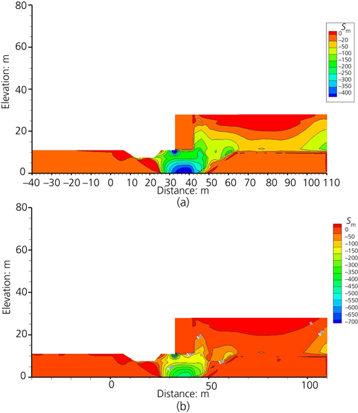
S m contours for SP soil, Ss = 0.99, T = 10 s, k s = 10−2 m/s, E = 40 MPa, (a) QS (b) PD result
S m contours for SP soil, Ss = 0.99, T = 10 s, k s = 10−2 m/s, E = 40 MPa, (a) QS (b) PD result
S m contours for SP soil, Ss = 0.99, T = 10 s, k s = 10−4 m/s, E = 20 MPa, (a) QS and (b) PD result
S m contours for SP soil, Ss = 0.99, T = 10 s, k s = 10−4 m/s, E = 20 MPa, (a) QS and (b) PD result
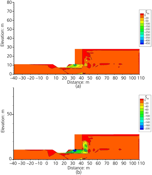
Effect of degree of saturation
This section presents the effect of saturation of seabed on liquefaction. The results are obtained under 10 s waves and for a particular seabed permeability of 10−4 m/s. The maximum amount of liquefaction occurs at different time values (or wave phases) in different regions. Three degrees of saturation are studied: 0.999, 0.995 and 0.980. Figure 21 shows that as the saturation of seabed decreases, the amount of liquefaction first increases in the backfill and then further decreases downwards, where there is little or no liquefaction in other regions.
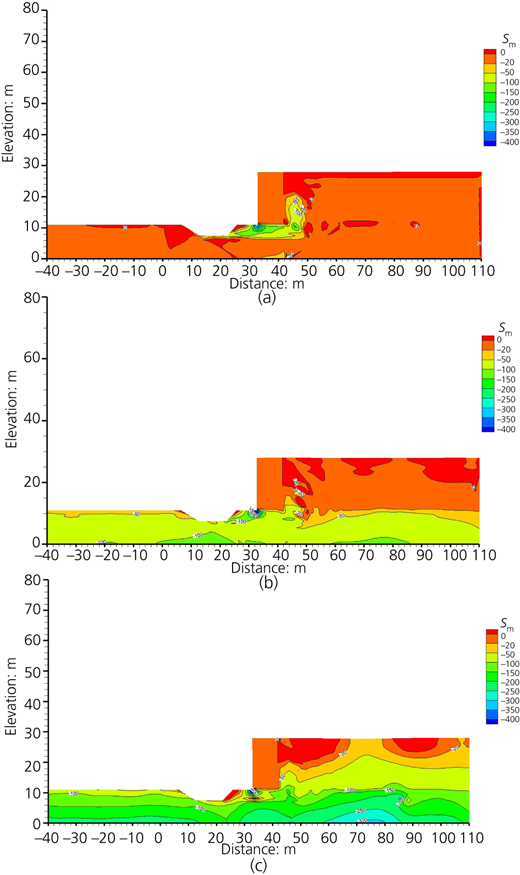
S m contours for SP soil, T = 10 s, k s = 10−4 m/s, E = 20 MPa, PD results for (a) Ss = 0.999, (b) Ss = 0.995, (c) Ss = 0.980 (units kPa)
S m contours for SP soil, T = 10 s, k s = 10−4 m/s, E = 20 MPa, PD results for (a) Ss = 0.999, (b) Ss = 0.995, (c) Ss = 0.980 (units kPa)
There is, however, calculated liquefaction potential along the seaward side as well as in the seabed for the 0.999 case (Figure 21(a)). In the analyses, the degree of saturation is naturally assumed to change just enough to provide air voids in the seabed, allowing mean stress reduction. It could be noticed that if the saturation decreases even slightly, the amount of liquefaction decreases in the seabed, which is in contrast to the backfill response where for lower saturations, an increase in liquefied regions is observed for T = 10 s (Figures 21(b) and 21(c)).
As the seabed degree of saturation decreases, the soil is more compressible (in both the foundation and the backfill), allowing less pore pressure development. This means that the seabed soil will be affected less by the CQW movement. This, in turn, causes slightly fewer areas in the backfill exhibiting tensile forces and thus causing less liquefaction. Also, there is little or no liquefaction in the foundation that can be attributed to this behaviour since a considerable amount of wave energy is absorbed by the contraction of seabed. It should also be noted that the backfill soil exhibits a considerable reduction in mean effective stress.
Effect of wave period
While investigating the effect of wave period on liquefaction potential, it is important to consider the change in wave properties such as wave steepness and wavelength, depending upon the water depth right at where the CQW is located. In this study, the wave parameters are considered on the evaluation of the dynamic response such that the wave forces acting on the CQW convey the maximum energy on the structure. Figure 22 presents that as the wave period increases, seabed soil exhibits more liquefaction. It is also observed that the interface between seabed and alluvial sloping ground both on the seaward side and in the backfill triggers liquefaction, irrespective of the wave period.
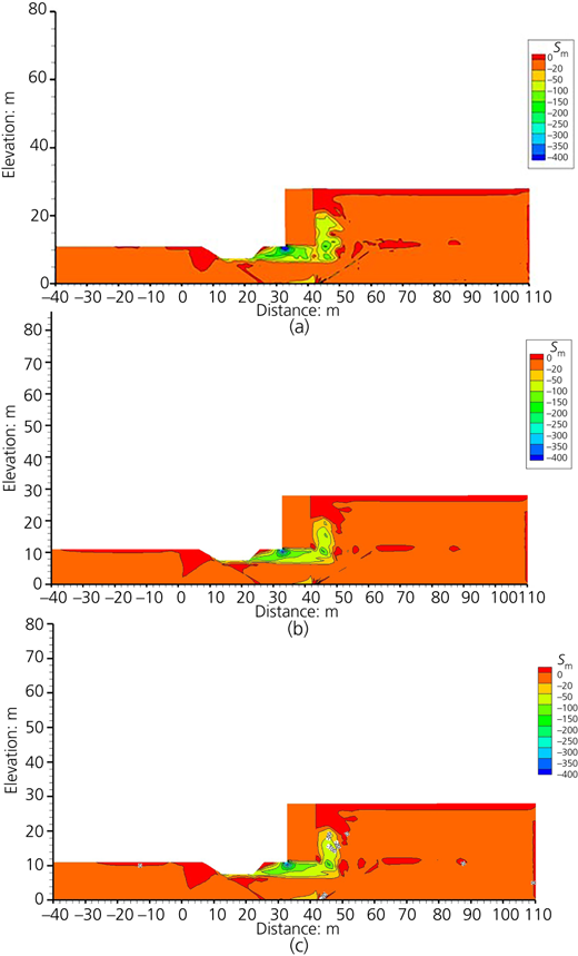
S m contours for SP soil, Ss = 0.99, k s = 10−4 m/s, E = 20 MPa, PD results (a) T = 5 s, (b) 7.5 s and (c) 10 s (units kPa)
S m contours for SP soil, Ss = 0.99, k s = 10−4 m/s, E = 20 MPa, PD results (a) T = 5 s, (b) 7.5 s and (c) 10 s (units kPa)
Shear behaviour
In another series of analyses, shear stress distributions are evaluated around the CQW. In soils, shear behaviour is evaluated by comparing the τs as the shear stress applied by the induced wave load on a particular plane and the τf as the shear strength of the soil in the same plane, which is a function of internal friction angle and possibly the cohesive strength. Since it is hard to determine the interface shear strengths of the components of the problem, one can assume that τf acts as the minimum value of such quantities across the plane section. The related variations of stress distribution provide useful information about the possible stress concentrations around the CQW.
Figure 23 presents the effect of inertial terms on the shearing resistance. There is more stress concentrations around the caisson in the PD analysis, making a greater difference between the inertial terms. Thus, the additional contribution comes from the incorporation of solid-phase motion.
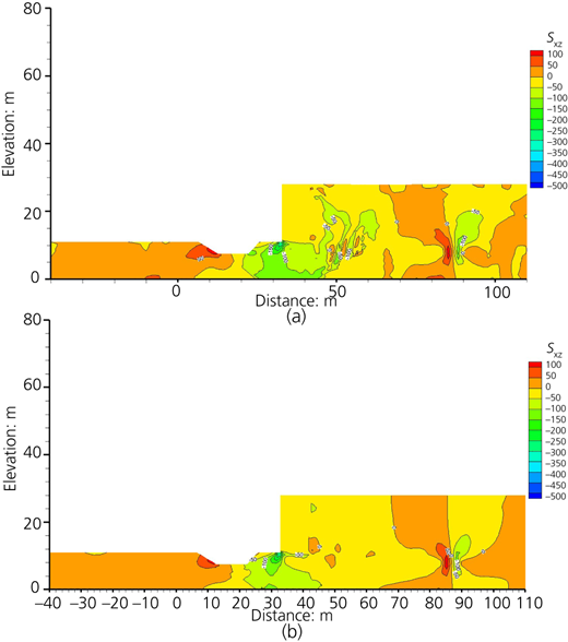
Sxz contours for SP soil, Ss = 0.99, ks = 10−2 m/s, E = 40 MPa, T = 5 s, (a) PD and (b) QS solution
Sxz contours for SP soil, Ss = 0.99, ks = 10−2 m/s, E = 40 MPa, T = 5 s, (a) PD and (b) QS solution
The effect of wave period on the shear behaviour is given in Figure 24. As the wave period decreases, the shearing effect on the dynamic response of the system increases. This is an important result; that below a certain period (i.e. 7.5 s in this study), a large amount of shear stresses are concentrated around the CQW. For T = 5 s, at a certain location from the wall, there is considerable stress development along a vertical plane between the seabed soil and the alluvial soil. It is observed that the non-uniform distribution of shear due to the rocking motion of the wall may localise such concentrations.
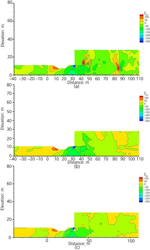
Sxz contours for SP soil, PD solution, Ss = 0.99, E = 20 MPa, ks = 10−4 m/s, (a) T = 5s, (b) T = 7.5 s and (c) T = 10s, (units kPa)
Sxz contours for SP soil, PD solution, Ss = 0.99, E = 20 MPa, ks = 10−4 m/s, (a) T = 5s, (b) T = 7.5 s and (c) T = 10s, (units kPa)
Conclusions
In this study, the wave-induced dynamic response and instability analysis of a deformable CQW, along with the surrounding seabed and backfill soils, are studied. The CQW is modelled as a porous material with very little permeability. The aim is to close the knowledge gap about the wave-induced CQW–seabed response without a breakwater in the vicinity, since the majority of the prior research has been done on quay walls considering earthquakes. As for results, soil displacements are localised around the CQW due to its rocking motion, thus creating localised stress concentrations. Displacements increase when the effect of dynamic terms is taken into account. Pore pressures rise around the CQW and decrease rather gradually in the rubble in the horizontal direction. The sudden and large decline of pore pressures at the back toe of the CQW point to the possible occurrence of a piping problem. As for the liquefaction potential, it depends highly on the amount of energy the CQW is being exposed to and how much of it is transferred to the seabed and the backfill. The larger the wave period is, the deeper and wider the liquefied regions get. Instantaneous liquefaction occurs between the alluvial slope and seabed, and there is considerable liquefaction potential in the backfill propagating downwards. Inertial terms affect the instantaneous liquefaction response, favouring mostly the PD formulation on the conservative side. Considering the Kobe port quay wall structure and its soil profile, it is indeed possible that such a wall–soil system is not just vulnerable to seismic liquefaction but also to wave-induced instantaneous liquefaction, affecting the entire CQW system as well. Such can be generalised for similar systems. Lastly, this work shows that the design and analysis of CQWs should account for the significant wave action that may be caused directly by the climate change in our time.
Acknowledgements
The authors appreciate the partial support by European Research Council through the Marie Curie Career Integration Grant, Dynamic Response and Instability of Seabed-Coastal Structure Systems under Waves, project #333831. The assistance of Dr. Mehran Hassanzadeh in the liquefaction analyses is also acknowledged.
