Mixing intensity and spatial strength variability in laboratory deep-mixed columns

$A*2$

Stephens-modified Anderson–Darling statistic

$C(0)$

sample variance of detrended residuals

$C(Δ)$

sample spatial covariance at lag $Δ$

$COVss$

within-slice COV

$d$

separation distance used in the autocorrelation model

$dij$

distance between measurement locations $i$ and $j$

$h$

horizontal lag distance

$lp(θ)$

profile log-likelihood function

$M$

total number of blade wings

$M*$

number of vertical profiles used in MLE

$N$

total number of measurement points per column

$NP$

needle penetration gradient (N/mm)

$Nd,Nu$

rotational speeds during downward and upward movements (rev/min)

$ns$

number of measurement points in slice $s$

$p$

probability value used in goodness-of-fit tests

$qu$

unconfined compressive strength, UCT (kPa)

$quNP$

converted UCT from needle penetration test (kPa)

$quNP,s,i$

converted strength at point $i$ in slice $s$

$q–uNP$

overall column mean of $quNP$

$q–uNP,s$

mean $quNP$ of slice $s$

$R(θ)$

exponential correlation matrix

$Rjk$

element of $R(θ)$

$S$

number of horizontal slices in a column

$T$

blade revolution count (rev/m)

$Vd,Vu$

downward and upward moving speeds of mixing blade (m/min)

$ws,i$

slice-mean-detrended residual at slice $s$⁠, position $i$

$zj,zk$

vertical coordinates of slices $j$ and $k$

$Δ$

spatial lag distance

$Δz$

vertical slice spacing

$ηh$

local horizontal variance ratio

$ηz$

depth-structured variance ratio

$θ$

exponential correlation-length parameter (cm)

$θv$

maximum likelihood estimate of vertical correlation length (cm)

$ρ(Δ)$

empirical autocorrelation function, ACF, at lag $Δ$

$ρ(d)$

theoretical ACF at separation distance $d$

$σ2$

process variance of exponential covariance model (kPa²)

$σh2$

local horizontal, variance of $quNP$ (kPa²)

$σtotal2$

total population variance of $quNP$ (kPa²)

$σu,s2$

within-slice population variance of slice $s$ (kPa²)

$σz2$

depth-structured, variance of $quNP$ (kPa²)

$σln$

lognormal spread parameter

The deep mixing method (DMM) is an in situ ground improvement technique in which cement slurry is mechanically mixed with soft soil to form stabilised columns. Column quality depends on the uniformity of cement distribution, which controls both the mean and variability of unconfined compressive strength, $qu$ (Zuo et al., 2023). Strength variability in DMM has been examined probabilistically since Honjo (1982) and later studies have developed statistical frameworks for interpreting core strength data, representative strength and design strength while accounting for variability, sample size and reliability criteria (Liu et al., 2008, 2017). More recent studies have shown that mean strength and standard deviation alone are insufficient because spatial correlation affects column behaviour and reliability (Namikawa, 2019; Namikawa and Koseki, 2013). Construction and mixing parameters also influence binder distribution and strength variability, although their effects on spatial correlation are not always consistent (Chen et al., 2016; Larsson et al., 2005; Zuo et al., 2023).

Existing characterisations commonly treat a DMM column as a single statistical population and report only the overall coefficient of variation (COV). This approach does not distinguish whether $qu$ variability is organised along the depth axis or scattered locally within horizontal cross-sections. The distinction is important because geotechnical variability is commonly described by both COV and spatial correlation structure, which govern how uncertainty is averaged over space in reliability-based design (Phoon and Kulhawy, 1999). In cement-treated columns, spatial autocorrelation can reduce the overall column strength relative to a uniform column with the same mean strength (Namikawa and Koseki, 2013), and the reliability of DMM column-supported embankments depends on mean strength, COV and spatial correlation length (Wijerathna and Liyanapathirana, 2019). Therefore, two columns with the same overall COV may require different interpretations if one is dominated by depth-structured variability and the other by local horizontal heterogeneity.

The blade revolution count $T$ (rev/m) is the principal mixing-intensity parameter in Japanese DMM practice. The rational mixing number concept of Ota et al. (2000) describes a threshold beyond which further increases in $T$ produce diminishing returns. However, how $T$ governs the internal spatial structure of $qu$ remains unclear. Although Chen et al. (2016) linked binder mass-fraction variability to strength variability and showed that improved mixing reduces overall COV, the partitioning of residual variability between depth-structured and local horizontal components has not been systematically examined.

This study forms part of a broader laboratory programme for evaluating DMM blade performance; however, the present paper focuses on one representative blade design operated at four blade revolution counts: T2, T4, T6 and T8, corresponding to 2000, 4000, 6000 and 8000 rev/m, respectively, with all other mix parameters held constant. Needle penetration tests at 20 positions on 11–12 slices per column provided spatially resolved values of $quNP$⁠, the converted unconfined compressive strength. Four complementary analyses are reported: (i) descriptive statistics of $quNP$⁠, establishing the mean and COV trends as a function of $T$⁠; (ii) decomposition of total $qu$ variance into depth-structured and within-slice components, an analysis that, to the authors’ knowledge, has not previously been applied to DMM strength data; (iii) parametric distribution fitting with formal goodness-of-fit testing; and (iv) spatial autocorrelation analysis with estimation of the vertical correlation length, interpreted within the broader geostatistical framework of scale-of-fluctuation estimation (Lloret-Cabot et al., 2014). Together these provide a more complete spatial characterisation of how mixing intensity governs DMM column quality than is achievable from overall COV alone.

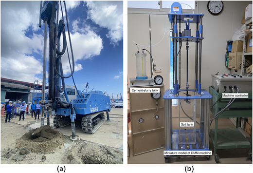
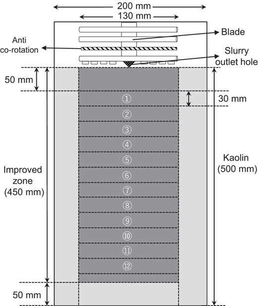
A miniature DMM apparatus was developed to reproduce the slurry-type mechanical mixing process under controlled laboratory conditions. Figure 1(a) shows a representative field-scale DMM machine, while Figure 1(b) shows the laboratory apparatus used in this study. Figure 2 shows the soil tank and experimental configuration. The apparatus comprises a mixing machine, cement-slurry delivery system and soil tank. The soil tank has internal dimensions of 200 mm × 200 mm in plan and 600 mm in height, and was filled with kaolin to a depth of 500 mm. Blade rotation speed can be controlled from 0 to 34 rpm, and vertical penetration and extraction speed from 0 to 1.0 m/min.

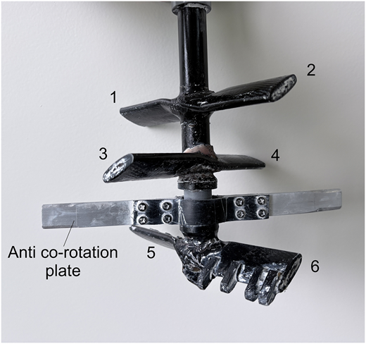
The mixing blade assembly is shown in Figure 3. It comprises six wings along a central shaft of 130 mm dia. (1/10 of a representative full-scale diameter of 1300 mm): four upper mixing wings to agitate the soil and distribute cement slurry, two lower cutting wings to assist penetration, and a horizontal anti-co-rotation plate to suppress co-rotation of the soil mass. Cement slurry was stored in a tank adjacent to the apparatus and delivered pneumatically through an internal conduit to the blade tip, where it was ejected into the surrounding soil. Ejection pressure was maintained at approximately 9 kPa. Since no flow meter was installed, slurry delivery was monitored by tracking the tank-level decrease against pre-calculated target values.

During each test, the blade was rotated and penetrated downward through the kaolin at the prescribed speed, with slurry ejected continuously throughout the 450 mm effective improved zone. On reaching the base, the rotation was reversed and the blade extracted upward at the same speed without further slurry ejection. The effective treated column diameter after mixing and curing was approximately 150 mm, slightly larger than the blade diameter owing to lateral soil displacement during rotation.

The base soil was prepared from powdered kaolin with a liquid limit of 66.6%, a plastic limit of 34.7% and a particle density of 2.61 mg/m³. Purified water was added to achieve a water content of 133.2%, equivalent to twice the liquid limit and corresponding to a liquidity index of 3.1. This high-fluidity condition was adopted for two reasons: it ensures uniform and reproducible filling of the soil box, minimising the influence of initial heterogeneity on the results; and the torque capacity of the miniature apparatus is limited, such that higher soil stiffness would have prevented adequate blade rotation. Although a water content of approximately 1.0–1.5 times the liquid limit is more representative of natural soft clay, the primary objective is to compare strength variability across mixing conditions rather than to reproduce absolute field behaviour.

The binder was a cement-based stabiliser, Solid Ace #100 (Aso Cement Co.), with a density of 3.13 mg/m³. A cement addition rate of 150 kg/m³ and a water-cement ratio of 1.5 were adopted for all mixing conditions. An admixture at 5% of dry cement content was included to enhance slurry fluidity and prevent outlet clogging. These proportions were held constant to isolate the effect of mixing intensity.

Mixing intensity was controlled through the blade revolution count, which is defined as the total number of blade passes per unit length of the improved zone during a single penetration and extraction cycle. Following the standard definition in Japanese DMM (Japanese Cement Association, 2021), $T$ is expressed as:

where $T$ is the blade revolution count (rev/m); $Nd$ and $Nu$ are the rotational speeds during downward and upward movements (rev/min), respectively; $Vd$ and $Vu$ are the downward and upward moving speeds of the mixing wings (m/min), respectively; and $M$ denotes the total number of blades composing the mixing wings. In the model tests, $M$ = 6 and $Vd$ = $Vu$= 0.051 m/min were fixed for all cases. The four mixing conditions examined in this study are summarised in Table 1. These cases are referred to as T2, T4, T6 and T8 corresponding to $T$ = 2000, 4000, 6000 and 8000 rev/m, respectively. The range of T from 2000 to 8000 rev/m was selected to span conditions from clearly under-mixed to very well-mixed states. All cases used identical soil preparation, cement type, cement dosage, slurry mix proportion and curing condition, so that differences in the resulting $qu$ distribution can be attributed solely to the difference in mixing intensity.

After mixing, each column was cured in the soil box at 20 ± 2°C for 7 days and then extracted. Each extracted column had a total length of approximately 450 mm and was cut into 11 or 12 horizontal slices of approximately 30 mm thickness using wire saws, starting from a depth of 50 mm. Exposed surfaces were smoothed with a straight blade knife to ensure reliable needle contact. Needle penetration tests were performed on each exposed surface in accordance with JGS 3431-2012 using a table-mounted device. The needle was pushed perpendicularly into the surface at a constant rate, and the applied load $P$ (N) and penetration depth $L$ (mm) were recorded until $L$ = 10 mm. The needle penetration gradient $NP$ (N/mm) was computed as $P/L$⁠, and the converted unconfined compressive strength $quNP$ was obtained from the empirical formula of Uchida et al. (2004):

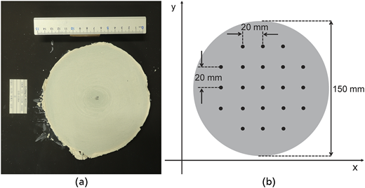
Figure 4(a) shows a typical exposed slice surface after cutting and smoothing. On each exposed surface, a square measurement grid with 20 mm spacing in both the x- and y-directions was established, as shown in Figure 4(b). The original grid comprised 21 points, but the centre point was excluded because cement tended to accumulate near the blade axis, giving a strength response unrepresentative of the surrounding mixed soil. The remaining 20 points were used at every slice depth and for all mixing conditions, ensuring spatial consistency throughout the dataset.

Table 2 summarises the overall statistical characteristics of the $quNP$ for the four mixing conditions. Each of T2, T4 and T6 comprised 240 measurements from 12 slices, whereas T8 comprised 220 measurements from 11 slices because slice 12 was lost during specimen extraction. The grand mean $quNP$ ranges from 136.5 kPa at T8 to 152.3 kPa at T4, with no monotonic trend, indicating that increasing blade revolution count mainly redistributes and homogenises strength rather than systematically increasing it. Overall COV decreases progressively from 0.168 at T2 to 0.089 at T8, consistent with improved mixing uniformity. Skewness also varies systematically. At T2, the distribution is moderately right-skewed (skewness = 0.68), indicating some locally high-strength zones. Skewness increases substantially at T4 and T6 (1.37 and 1.42, respectively), reflecting extreme high-strength values and, for T6, distributional distortion arising from the depth-wise strength gradient. At T8, skewness approaches zero (−0.15), consistent with near-uniform mixing.

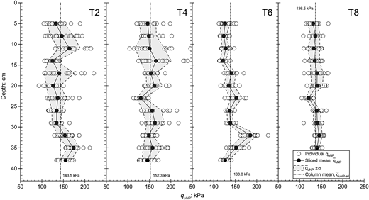
Figure 5 shows the vertical distribution of $quNP$ for the four mixing conditions; Table 3 presents, for each case, the depth-wise range of slice means and the within-slice coefficient of variation COV_ss, computed from the 20 measurement points within each horizontal test plane. Two distinct variability patterns emerge. At T2 and T4, COV_ss is high and varies substantially between slices. At T2, five of the 12 slices have COV_ss exceeding 0.15 (maximum 0.246), reflecting incomplete cement dispersion across the horizontal cross-section. At T4, two slices exceed COV_ss = 0.15 (maximum 0.234), with individual values reaching 245.8 kPa, the maximum recorded.

At T6, within-slice uniformity improves markedly: all 12 slices show COV_ss below 0.10 (range 0.043–0.094, mean 0.070). However, slice means vary substantially with depth, from 121.4 kPa at 15.5 cm to 184.9 kPa at 33.5 cm, a depth-wise range of 63.5 kPa, the largest across all four cases. This pattern of low within-slice scatter combined with large depth-wise variation in slice means is the defining characteristic of the T6 case and is examined in detail in Section 4. At T8, both aspects of variability are minimised simultaneously. All slices have COV_ss below 0.11 (range 0.042–0.105, mean 0.074) and the slice-mean range narrows to only 24.6 kPa, confirming near-uniform cement distribution in both the horizontal and vertical directions.

Overall, COV decreases monotonically with $T$ but cannot distinguish a column dominated by local horizontal heterogeneity (T2, T4) from one whose cross-sections are individually uniform but differ systematically with depth (T6). Section 4 decomposes total variance into depth-structured and local horizontal components to quantify this distinction.

Total $quNP$ variance within each column was decomposed into a depth-structured component, reflecting systematic differences in mean strength between depth levels, and a local horizontal component, reflecting point-to-point scatter within each horizontal test plane. Denoting total population variance as $σtotal2$⁠, the decomposition is:

where$σz2$ is the depth-structured (between-slice) variance and $σh2$ is the local horizontal (within-slice) variance, defined, respectively, as:

Here, $S$ is the number of slices, $ns$ is the number of measurement points in slice $s$⁠, $N$ is the total number of measurement points, $quNP,s,i$ is the converted strength at point $i$ in slice $s$⁠, $q–uNP,s$ is the mean strength of slice s, and $q–uNP$ is the overall column mean. The variance ratios are defined as:

where $ηz$ quantifies the proportion of total $quNP$ variance attributable to depth-level mean differences, whereas $ηh$ quantifies the proportion attributable to local horizontal heterogeneity within each test plane. Both ratios are expressed as percentages to compare cases with different absolute variances.

Since each mixing condition is represented by a single physical column, the point estimates of $ηz$ and $ηh$ describe the individual model columns rather than the population of all DMM columns produced under each T setting. Hierarchical bootstrap 95% confidence intervals are reported alongside the decomposition results in Table 4, computed by resampling slices with replacement and, within each resampled slice, resampling measurement points with replacement (2000 replications). The intervals are wide owing to the small number of slices per column, but the rank ordering of cases by $ηz$ is preserved across the full bootstrap distribution.

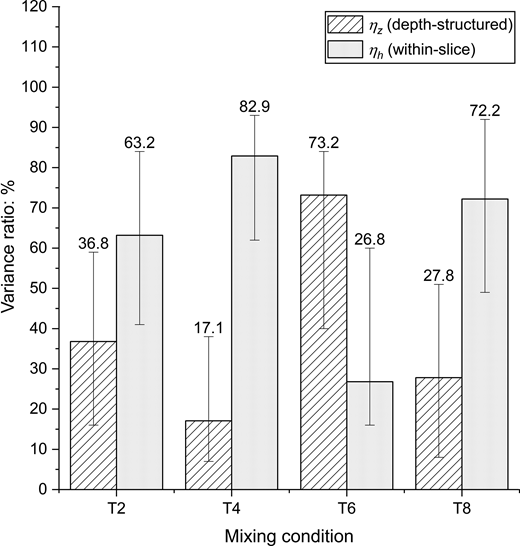
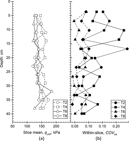
Figure 6 shows the variance ratios as a stacked bar chart; Figures 7(a) and 7(b) show depth profiles of slice-mean $quNP$ and within-slice COV_ss, respectively. Three distinct regimes are identified. At T2, local horizontal heterogeneity dominates (⁠$ηh$ = 63.2%), with COV_ss spanning 0.077–0.246, reflecting insufficient mixing to homogenise cement distribution within each cross-section. At T4, local dominance intensifies (⁠$ηh$ = 82.9%), making T4 the most locally heterogeneous case despite its moderate overall COV of 0.148.

The most striking result occurs at T6, where $ηz$ reaches 73.2%, the highest depth-structured ratio across all cases, while COV_ss remains consistently tight (0.043–0.094). Slice means nevertheless vary substantially with depth (121.4–184.9 kPa, range 63.5 kPa), demonstrating that within-slice homogeneity does not guarantee depth-wise uniformity. The mechanism responsible for this depth-wise gradient at T6 is identified as a subject for further investigation.

At T8, total variance falls to 145.8 kPa², less than one quarter of the T2 value, with both components substantially reduced and the slice-mean range narrowing to 24.6 kPa. The non-monotonic behaviour of $ηz$ (36.8% → 17.1% → 73.2% → 27.8%) indicates that within-slice homogeneity is largely achieved near T6, while depth-wise uniformity is not fully established until T8, broadly consistent with the rational mixing number concept of Ota et al. (2000), but adds a spatial interpretation to the mixing threshold. Reporting $ηz$ and $ηh$ alongside overall COV therefore provides a more complete description of column quality.

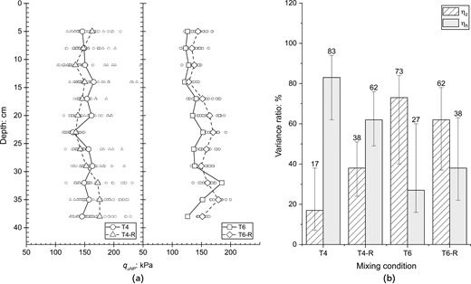
Two additional columns were prepared under the T4 and T6 conditions to assess repeatability; the replicates are denoted T4-R and T6-R. Numerical comparisons are summarised in Table 5, and depth profiles and variance-decomposition results are shown in Figure 8. Mean $quNP$ is reproduced closely for T4 (152.3 vs. 152.7 kPa) but less so for T6 (138.8 vs. 152.4 kPa). Overall COV differs by only 0.008 between T4 replicates and 0.024 between T6 replicates, indicating good reproducibility of global variability magnitude.

In contrast, the variance partitioning shows greater between-column variability. For T4, $ηz$ increases from 17.1% in T4 to 38.1% in T4-R; for T6, $ηz$ decreases from 73.2% in T6 to 62.3% in T6-R. Despite these differences, the rank ordering is preserved: both T6 columns exhibit higher $ηz$ than both T4 columns, indicating that the qualitative distinction between locally heterogeneous behaviour at T4 and more depth-structured behaviour at T6 is reproducible.

The hierarchical-bootstrap 95% confidence intervals in Table 5 partly overlap, so the replicate comparison does not constitute a formal statistical separation. Nevertheless, the consistent rank ordering supports the interpretation that mixing intensity governs the spatial character of variability, not only its magnitude. The T4 vs. T4-R contrast suggests that variance partitioning is sensitive to factors not fully controlled by the present apparatus, potentially including local fluctuations in slurry-delivery pressure. This does not invalidate the qualitative findings but indicates that single-column estimates of $ηz$ and $ηh$ may carry inter-column uncertainty of approximately 10–20 percentage points. Replicate columns are therefore recommended in future studies.

The variance decomposition in Section 4 showed that mixing intensity changes not only the magnitude of $quNP$ variability but also its spatial organisation. This section examines whether these changes are also reflected in the probability distribution of $quNP$⁠. This is important because DMM design and quality-control practice recognise substantial scatter in in situ treated-soil strength and require correction factors to account for this variability (CDIT, 2002), while probabilistic assessments of representative/design strength depend on the adopted statistical model and lower-tail criteria (Liu et al., 2017). In addition, uncertainty in the estimated strength parameters depends on sample size and spatial correlation (Namikawa, 2019).

Normal and Lognormal distributions were fitted by maximum likelihood. These distributions were selected because both have been examined in previous statistical studies of cement-treated soil strength, although neither should be assumed universally applicable without goodness-of-fit checking (Liu et al., 2017; Namikawa and Koseki, 2013). The normal distribution was tested as a symmetric benchmark that may become appropriate under relatively uniform mixing conditions, whereas the Lognormal distribution was tested as a positive-valued, right-skewed alternative for heterogeneous strength data. Goodness of fit was assessed using the Lilliefors-corrected Kolmogorov–Smirnov test (Lilliefors, 1967) and the Stephens-modified Anderson–Darling test (Stephens, 1974, 1976) at $α$ = 0.05. A distribution was treated as acceptable only when it passed both corrected tests simultaneously.

Distributions were also fitted to slice-mean-detrended residuals, $ws,i=quNP,s,i-q–uNP,s$⁠, to determine whether apparent non-normality originates from the depth-trend structure or from the local residual field. Because these residuals are spatially nested within slices rather than strictly independent, the detrended $p$-values should be interpreted as descriptive screening metrics, not exact significance tests.

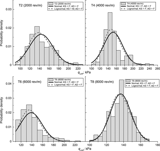
The test results are summarised in Table 6. Histograms with fitted probability density functions are shown in Figure 9. At T2, the normal distribution is rejected by both tests $KS p$ = 0.0010; $AD A*2$ = 2.211, $p$ < 0.01. The Lognormal distribution gives a marginal fit, passing the KS test (⁠$p$ = 0.059) and falling near the AD acceptance threshold (⁠$A*2$ = 0.768, $p$ = 0.05–0.10). However, this should not be interpreted as strong evidence of Lognormal behaviour because the distribution remains right-skewed and tail-sensitive. This is consistent with $ηh$ = 63.2%, where local within-slice heterogeneity produces isolated high-strength zones that generate right-skewed behaviour (skewness = 0.68). Slice-mean detrending does not restore normality (⁠$KS p$ = 0.0075; $AD p$ < 0.01), suggesting that the local residual field remains non-Gaussian at T2.

At T4, both distributions are rejected for the raw data. Strong right skew (skewness = 1.37) and extreme values reaching 245.8 kPa produce a heavy-tailed distribution that neither model adequately represents. The high $ηh$ = 82.9% suggests that isolated high-strength zones remain within individual cross-sections, generating outliers that distort the distribution. Slice-mean detrending also fails to produce normal residuals (⁠$KS p$ = 0.0010; $AD p$ < 0.01), indicating that the local residual field remains strongly non-Gaussian.

At T6, both distributions are rejected for the raw data. The histogram does not show a simple unimodal distribution and instead exhibits a pronounced right tail associated with large differences in slice-mean strength. This behaviour is consistent with pooling slices whose means span 121.4–184.9 kPa and with the high depth-structured variance ratio (⁠$ηz$ = 73.2%) identified in Section 4. After slice-mean detrending, the departure from a simple normal form is reduced and the KS test no longer rejects normality. This indicates that the poor fit of the raw T6 distribution is mainly associated with depth-wise variation in slice means rather than the local residual field alone. The AD test, however, continues to reject the detrended residuals, indicating that residual tail mismatch remains.

At T8, the raw dataset is the only case for which the normal distribution is not rejected by either test at $α$ = 0.05. The near-zero skewness and low COV are consistent with near-uniform mixing. The T8 dataset is slightly smaller (⁠$n$ = 220), which marginally reduces test power; therefore, the acceptance of normality should be treated as suggestive rather than definitive. For the slice-mean-detrended T8 residuals, the KS test does not reject normality (⁠$p$ = 0.1330), but the AD test remains marginally sensitive to tail mismatch (⁠$A*2$ = 0.873, $p$ = 0.025–0.05); therefore, the detrended T8 residuals are treated as a KS pass but not a full normal fit.

The lognormal spread parameter decreases monotonically with increasing T, from $σln$ = 0.164 at T2 to 0.145 at T4, 0.142 at T6, and 0.090 at T8, confirming that distributional spread narrows with increasing $T$⁠. However, because the lognormal distribution is rejected or only marginally supported for T2–T6, this parameter should be interpreted as a descriptive measure of log-scale spread rather than a structural distributional parameter. Overall, the conventional lognormal assumption is not consistently supported in the present miniature-column dataset. Only T8 provides tentative support for a normal approximation. More importantly, distribution shape reflects the spatial organisation of strength: the distorted T6 distribution is mainly associated with depth-wise mean variation, whereas the near-normal T8 distribution reflects the simultaneous reduction of both spatial variance components. Overall COV alone is therefore insufficient to characterise DMM column quality.

The spatial autocorrelation structure of $quNP$ was examined in the horizontal and vertical directions using slice-mean-detrended residuals. This detrending was applied to remove the depth-structured component identified in Section 4, so that the ACF analysis represents the residual spatial structure of the local $quNP$ field. This follows the geostatistical treatment in which spatial variability is separated into a deterministic trend and a residual component characterised by variance and autocorrelation structure (Baecher and Christian, 2003; Vanmarcke, 1977). For each measurement point at slice $s$ and horizontal position $i$⁠, the detrended residual is defined as:

where $q–uNP(s)$ is the mean of the 20 measurement points within slice s. The empirical autocorrelation function (ACF) was computed as:

where $C(Δ)$ is the sample covariance between all pairs of residuals separated by lag $Δ$⁠, and $C(0)$ is the sample variance. Horizontal pairs were formed from measurement points within the same slice, whereas vertical pairs were formed from corresponding horizontal positions across different depth levels and pooled across the 20 vertical profiles. For the vertical direction, the one-dimensional exponential covariance model was adopted following Vanmarcke (1977):

or equivalently in correlation form, following Honjo (1982):

where $h$ is the vertical lag distance, $σ2$ is the process variance and $θ$ is the exponential correlation-length parameter. The exponential form was selected because it provides a simple single-parameter representation of spatial correlation and has been widely used in geotechnical random-field modelling (Baecher and Christian, 2003; Vanmarcke, 1977), including cement-treated soil strength data (Honjo, 1982; Namikawa, 2019; Namikawa and Koseki, 2013).

The vertical correlation length $θv$ was estimated by maximum likelihood, following the multivariate-normal covariance formulation of DeGroot and Baecher (1993) and Namikawa and Koseki (2013). The 20 vertical profiles at distinct horizontal positions were treated as approximately exchangeable realisations of the residual vertical random field. This is a simplifying assumption because all profiles were obtained from a single laboratory column. However, a one-way analysis of variance of mean $quNP$ against radial distance from the grid centre showed no statistically significant radial trend for any mixing condition (p > 0.05), supporting this approximation. For each vertical profile $i$⁠, the vector of $ns$ detrended residuals was modelled as a multivariate normal vector with zero mean and covariance $σ2R(θ)$⁠, where $R(θ)$ is the $ns×ns$ correlation matrix with elements:

where $zj$ and $zk$ are the depth centre coordinates of slices $j$ and $k$⁠, respectively. The matrix $R(θ)$ was decomposed using the Cholesky factorisation $R = LLT$ for numerical stability, avoiding direct matrix inversion. Treating the 20 profiles as independent, the total profile log-likelihood obtained by analytically eliminating $σ2$ is:

where $M*$ = 20 is the number of vertical profiles and $ns$ is the number of slices in each profile. For any given $θ$⁠, the profile estimate of the variance is:

The MLE of the vertical correlation length is then:

obtained by evaluating $lp (θ)$ over a fine grid of candidate values. The 95% confidence interval for $θv$ was computed using the profile likelihood ratio criterion. All values of $θv$ satisfying

are included in the interval, where 1.921 = $χ1,0.952/2$ corresponds to half of the 5% upper-tail critical value of the chi-squared distribution with one degree of freedom.

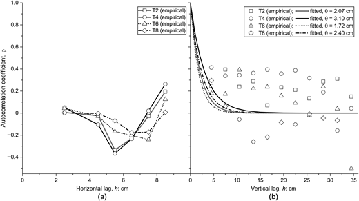
The empirical ACF profiles are shown in Figure 10, and the MLE results for the vertical correlation length are summarised in Table 7. After slice-mean detrending, the horizontal ACF values are effectively zero for all mixing conditions. The maximum correlation across all cases and horizontal lags is only 0.049, which is within the range of sampling noise. Thus, no meaningful horizontal spatial correlation is detectable at the present measurement scale. Because the horizontal grid spans only 8 cm and the inter-point spacing is 2 cm, this result should be interpreted as a resolution-limited finding, not as evidence that horizontal correlation is absent in general.

The detrended vertical ACF profiles show positive but irregular short-lag correlations. The fitted vertical correlation lengths range from 1.72 to 3.10 cm. T4 gives the longest value (⁠$θv$ = 3.10 cm), indicating the greatest residual vertical continuity after detrending. This is consistent with its high within-slice heterogeneity, because unresolved local strength zones may extend slightly across the 3 cm slice boundaries. T6 gives the shortest value (⁠$θv$ = 1.72 cm), consistent with its more homogenised within-slice structure and weak residual continuity beyond the nearest measurement depth.

All estimated $θv$ values are comparable to, or smaller than, the 3.0 cm slice spacing. The MLE estimates are therefore weakly constrained, and the confidence intervals are correspondingly wide (Lloret-Cabot et al., 2014). Because autocorrelation-distance estimates may be biased under limited-data conditions and are sensitive to the assumed correlation function (Cami et al., 2020; Qi and Liu, 2019), the values in Table 7 should be regarded as approximate order-of-magnitude estimates. Finer vertical sampling would be required for more reliable $θv$ estimation.

The estimated laboratory values are much smaller than reported field-scale vertical correlation parameters. Honjo (1982) reported vertical autocorrelation distances of approximately 0.4–4.0 m for cement-stabilised soil. Al-Naqshabandy et al. (2012) reported vertical scales of fluctuation of 0.2–0.7 m for lime-cement columns, corresponding to exponential correlation lengths of approximately 0.1–0.35 m. Pittaro and Mace (2024) reported vertical scales of fluctuation of approximately 0.5–3.5 m for DMM in the Kallang formation, corresponding to approximate exponential correlation lengths of 0.25–1.75 m under the same convention. These values are several times to two orders larger than the present estimates of $θv$ = 1.72–3.10 cm. Direct transfer of $θv$ from the miniature tests to field conditions is therefore inappropriate.

Overall, the dominant spatial structure is the depth-wise mean gradient identified by the variance decomposition, rather than a residual random field with substantial correlation length. Once the depth trend is removed, the residual $quNP$ field approaches spatially uncorrelated behaviour at the scale of the present measurement grid.

Although these numerical values are specific to the present tests, the framework itself is not inherently tied to the specimen scale or base material, provided that spatially referenced strength data are available. In the field, the needle-penetration values used here could be replaced by strength data from cored samples or suitable in situ measurements such as cone penetration tests, which have been used to characterise strength variability in lime-cement columns (Al-Naqshabandy et al., 2012). Measurements at multiple positions across the column diameter over several depths would provide the within-depth variability used to estimate the local horizontal component $σh2$⁠, whereas differences among the corresponding depth-level mean strengths would provide the depth-structured component, $σz2$⁠. Applying the variance decomposition of Section 4 would therefore indicate whether field-column variability is predominantly depth-structured or locally horizontal, with the former warranting denser vertical sampling and the latter greater cross-sectional coverage. The numerical values and appropriate sampling intervals would nevertheless need to be established from field-scale data and site conditions.

The internal strength variability of laboratory deep-mixed columns was characterised across four blade revolution counts, T2–T8, using descriptive statistics, variance decomposition, distribution fitting and spatial autocorrelation analysis. The main findings are summarised below.

• Mean $quNP$ did not vary monotonically with blade revolution count, whereas overall COV decreased from 0.168 at T2 to 0.089 at T8. Under the present laboratory conditions, increasing mixing intensity mainly reduced strength variability rather than increasing mean strength.

• Variance decomposition identified distinct spatial patterns. T2 and T4 were dominated by local horizontal heterogeneity (⁠$ηh$ = 63%–83%), whereas T6 was dominated by depth-structured variability (⁠$ηz$ = 73%). At T8, total variance fell to less than one quarter of the T2 value and the slice-mean range narrowed substantially. Thus, within-slice homogeneity and depth-wise uniformity did not develop simultaneously with increasing mixing intensity.

• Normal and lognormal fits were not consistently supported. Raw $quNP$ distributions at T4 and T6 were rejected by both models, T2 showed only marginal lognormal support, and the poor T6 fit mainly reflected depth-wise variation in slice means. Only T8 provided tentative support for a normal approximation.

• Detrended horizontal autocorrelation was effectively zero at the present grid resolution. Detrended vertical correlation lengths were 1.72–3.10 cm, comparable to the 3.0 cm slice spacing, indicating that the dominant spatial structure was the depth-wise mean variation rather than a strongly correlated residual field.

Overall, COV alone is an incomplete descriptor of DMM column quality. Columns with high $ηz$ require denser vertical sampling, whereas those with high $ηh$ require greater horizontal coverage. Reporting $ηz$ and $ηh$ alongside COV provides a more informative characterisation of strength variability. It may also support future comparison of alternative blade geometries in terms of depth-wise uniformity and local horizontal heterogeneity.

The authors gratefully acknowledge the GI Column Association for providing the miniature DMM apparatus and funding support for the experimental programme. The authors also thank Mr. Shota Sato for assisting with the laboratory experiments.