

This paper aims to obtain accurate forecasts of the hourly residential natural gas consumption, in Egypt, taken into consideration the volatile multiple seasonal nature of the gas series. This matter helps in both minimizing the cost of energy and maintaining the reliability of the Egyptian power system as well.
Double seasonal autoregressive integrated moving average-generalized autoregressive conditional heteroskedasticity model is used to obtain accurate forecasts of the hourly Egyptian gas consumption series. This model captures both daily and weekly seasonal patterns apparent in the series as well as the volatility of the series.
Using the mean absolute percentage error to check the forecasting accuracy of the model, it is proved that the produced outcomes are accurate. Therefore, the proposed model could be recommended for forecasting the Egyptian natural gas consumption.
The contribution of this research lies in the ingenuity of using time series models that accommodate both daily and weekly seasonal patterns, which have not been taken into consideration before, in addition to the series volatility to forecast hourly consumption of natural gas in Egypt.
1. Introduction
Natural gas constitutes one of the keystones of both economic and social development, as it plays an essential role in reducing pollution and maintaining environmental cleanness. It is commonly used for many purposes such as heating, electricity generation, transportation, cooking and cooling. All these usages give it a wide prominence in economic, social and technological developments in any country.
Pursuant to the energy information administration of the USA, Egypt is one of the largest natural gas producers in the continent. However, it is worth noting that, during the past two decades, Egyptian total demand for energy has grown at an annual rate of 4.6% and there is an expectation for more increase. Consequently, adopting energy management policies becomes very essential (African Development Bank Group, 2010).
It is well-known that decision-makers, around the world, widely use scientific forecasting methods for making such a scientific plan for development. Policymaking in the field of natural gas is not an exception. For instance, determining accurate forecasts of natural gas consumption for one day ahead is crucial for the economical and reliable operation of the distributed network.
Natural gas consumption is mainly influenced by seasonal effects (daily and weekly cycles as well as calendar holidays) and could be classified into three main types; residential, industrial and commercial consumption. The fundamental features of these types usually differ owing to the fact that each type has a seasonal cycle related to its characteristics. For instance, residential consumption is expected to increase at weekends compared to working days. While both commercial and industrial consumption is expected to increase on working days.
Moreover, it is very important to clarify that multiple seasonal patterns are also apparent in the Egyptian residential gas consumption series. In this context, it can be seen, through the series, that daily seasonal pattern is apparent in the similarity of hourly consumption from one day to the next, while a weekly seasonal pattern is apparent in the similarity of the daily consumption existing week after week. Accordingly, a double seasonal autoregressive integrated moving average (DSARIMA) model can be used to capture those seasonal patterns. Furthermore, the generalized autoregressive conditional heteroskedasticity (GARCH) model may be also used to capture the conditional volatility heteroskedasticity observed in the series.
Consequently, in this study, a DSARIMA-GARCH model is used to study the Egyptian hourly residential natural gas consumption. The DSARIMA model is used to accommodate both daily and weekly seasonal patterns whereas the conditional volatility behavior is captured by the GARCH model. The remainder of this research is organized as follows; Section 2 reviews the previous studies investigating the usage of autoregressive integrated moving average (ARIMA) model in forecasting gas consumption, Section 3 describes the Egyptian residential gas consumption series followed by an illustration of the DSARIMA-GARCH model in Section 4. In Section 5, the proposed model of the Egyptian gas consumption is introduced while Section 6 concludes the study and clarifies some points to be studied in the future.
2. Literature review
ARIMA models are extensively used in forecasting based on previously observed values of a time series. It has been used, in many preceding studies, to obtain accurate forecasting of natural gas consumption. In this part, an investigation of some studies is introduced to clarify the essential role of this model in making an accurate forecasting.
In their study, Liu and Lin (1991) used the ARIMA model to forecast natural gas consumption in Taiwan. The model was used with some exogenous variables such as temperature and prices. The study was conducted based on monthly data and monthly as well as quarterly forecasts were obtained. In 2004, the ARIMA model was used with the sake of forecasting the natural gas consumption in some residential areas of Eskisehir in Turkey. Based on a monthly data, the ARIMA model was used with separate autoregressive (AR) models to estimate both heating and non-heating months to capture the seasonal patterns (Aras and Aras, 2004). In his research, Al-Fattah (2006) adopted the use of ARIMA models to predict the USA natural gas production and annual depletion.
In 2010, the ARIMA models were used to forecast monthly Turkish natural gas consumption based on monthly data covering the period from 1987 to 2007 (Erdogdu, 2010). Moreover, Akkurt et al. (2010) used the Seasonal ARIMA (SARIMA) model, which is an extension of ARIMA model, in a comparative study with the linear regression model to forecast Turkish natural gas consumption in a monthly and yearly base through a time-series data having single seasonal pattern.
In their study, SARIMA model provided better results compared with the regression model. In other words, the values of the mean absolute percentage error (MAPE) and the mean absolute deviation of the forecasts that produced from time series models were lower than those corresponding of the linear regression. Furthermore, based on the historical monthly gas consumption, in Bangladesh, during the period (1980–2008), the ARIMA model was used to estimate the gas consumption in 2014 (Faisal, 2012).
Recently, different statistical methods among ARIMA models are used, in two studies, to forecast natural gas consumption in Turkey using residential and commercial data. The results of these studies demonstrate the use of ARIMA models to obtain an accurate natural gas consumption forecasting (Taspinar et al., 2013; Akpinar and Yumusak, 2016).In addition, they are also proved to be accurate in forecasting gas consumption in India and Iran (Pradhan et al., 2016; Jafari and Sadigh, 2019).
ARIMA model is not used to forecast the Egyptian gas consumption. In addition, the volatile multiple seasonal nature of the gas series is not taken into consideration in the previous studies. Hence, DSARIMA, as an extension of ARIMA model, is used in this study to accommodate daily and weekly seasonal patterns and combined with GARCH model to capture the volatility of the series to obtain accurate forecasts of the Egyptian residential gas consumption.
3. Egyptian natural gas consumption series
The residential natural gas consumption, in Egypt, is analyzed based on hourly data of a one year, specifically from the first Sunday (1st of January) to the last Sunday (31th of December) of 2017. All the data, with 8,760 hourly observations, is used to estimate the model. In this context, it is worth noting that the first month of 2018, with 744 hourly observations, is also obtained for the sake of being used to evaluate the forecasting accuracy of the model.
Figure 1 presents a time series plot of a part of the data. It clarifies the Egyptian hourly residential gas consumption series from Wednesday, 1 March 2017, to Friday, 31 March 2017. It can be seen that hours from 1 to 24 represent the 24 h of the first day of this part of the time series while the hours from 24 to 48 illustrate the second day, etc. A typical daily seasonal pattern is apparent in the similarity of the consumption from one day to the next. Moreover, a weekly seasonal pattern is apparent as well. It can be shown that working days show similar patterns of consumption, while weekends have different natural gas consumption. Weekends have a residential natural gas consumption, that is higher than the corresponding of the working days.
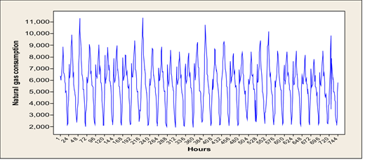
Time plot of the Egyptian hourly gas consumption series from Wednesday 1 March 2017 to Friday 31 March 2017
Time plot of the Egyptian hourly gas consumption series from Wednesday 1 March 2017 to Friday 31 March 2017
4. Double seasonal autoregressive integrated moving average-generalized autoregressive conditional heteroskedasticity model
DSARIMA-GARCH models are used to model time-series data that contains two seasonal cycles. This can be conducted by representing the current values of the series as a combination of past seasonal values and past seasonal errors. However, this is with the condition that there are one or more observations, in the series, for which the variance of the current error term is a function of the previous time periods’ error or previous error variance.
A DSARIMA-GARCH model, which can be denoted as ARIMA (p,d,q)(P1,D1,Q1)s1(P2,D2,Q2)s2−GARCH(r,s), could be written as:
with error term εt splits into a stochastic piece ηt and a time-dependent standard deviation σt so that:
where ηt is independent and identical distributed with zero mean and variance equal to one and is modeled as follows:
yt is a time series, s1 and s2 are the first and second seasonal periods,∇d is the nonseasonal differencing operator while is the seasonal differencing operator; B is the backward shift operator such that Biyt = yt−1; ϕp(B) represents the nonseasonal AR polynomial of order p and θq(B) represents the nonseasonal moving average polynomial of order q, likewise ΦP1(Bs1) and ΩP2(Bs2) are seasonal AR polynomials of orders P1 and P2 for the first and second seasonal cycles respectively; and ΘQ1(Bs1) and ΨQ2(Bs2) are seasonal moving average polynomials of orders Q1 and Q2 respectively. r is the order of the GARCH terms and s is the order of the ARCH terms.
4.1 Double seasonal autoregressive integrated moving average model
The multiplicative SARIMA model has been introduced by Box and Jenkins (1976) to capture only one seasonal pattern. SARIMA model is denoted as ARIMA (p, d, q) (P, D, Q)s where p and P are the number of non-seasonal and seasonal AR terms respectively, d is the order of the difference needed to render stationarity while D is the order of seasonal differencing, q is the number of moving average terms that represent the past errors, Q is the number of seasonal moving average terms and s is the seasonal period. SARIMA model could be expressed as:
SARIMA model has been extended to DSARIMA model by Taylor (2003) to accommodate two seasonal patterns (daily and weekly). Therefore, second seasonal AR and moving average terms and second seasonal differencing operator have been added to SARIMA model. The multiplicative DSARIMA model, which is denoted as ARIMA (p, d, q) (P1, D1, Q1)s1 (P2, D2, Q2)s2, is expressed as follows:
4.2 Generalized autoregressive conditional heteroskedasticity model
In his research, Engle (1982) introduced the autoregressive conditional heteroscedasticity (ARCH) model that has been extended later by Bollerslev (1986) to the GARCH model. The ARCH model assumes that the conditional variances of the error are described by a function of previous squared errors and could be used when the error variance is assumed to follow AR model. To model a time series using an ARCH process, let εt denote the error term. This εt consists of a stochastic piece ηt and a time-dependent standard deviation σt as follows:
where ηt ∼ N (0, 1) i.i.d. Then, is modeled by:
GARCH model is a generalization of ARCH model. It is used when the error variance assumed to follow autoregressive moving average model (ARMA) model. The conditional variance is not only explained by past squared errors but also by past conditional variances. The GARCH (r, s) model for a series yt is given by:
4.3 Properties of double seasonal autoregressive integrated moving average-generalized autoregressive conditional heteroskedasticity model
Stationarity and invertibilty are important concepts in analyzing time series. A time series that follows DSAIMA-GARCH model is stationary if the absolute roots of the nonseasonal and seasonal AR polynomials ϕp(B) = 0,ΦP1(Bs1)=0 and ΩP2(Bs2)=0 are greater than 1.While invertibility is a model characteristic on the contrary to stationarity, which is a time series characteristics. DSARIMA-GARCH model is invertible if the absolute roots of the nonseasonal and seasonal moving average polynomials θq(B) = 0, ΘQ1(Bs1)=0 and ΨQ2(Bs2)=0 are greater than 1 (Box et al., 1994).
In other words, there are several constraints on the parameters of the DSARIMA-GARCH model. The roots of the polynomials ϕp(B),ΦP1(Bs1), ΩP2(Bs2), θq(B), ΘQ1(Bs1) and ΨQ2(Bs2) should be outside the unit circle to satisfy the sationarity and invertibility conditions for the DSARIMA part, while the constrains αi > 0, i = 0, …, s and βj > 0, j = 1, …, r are assumed to guarantee the positivity of the conditional variance for the GARCH part (Bollerslev, 1986; Brooks, 2008; Tsay, 2010).
5. Empirical results
Different DSARIMA-GARCH models are estimated to forecast hourly residential natural gas consumption in Egypt. Firstly, to identify a suitable DSARIMA model, the estimated autocorrelation function (ACF) of the Egyptian consumption series is plotted. The ACF is a tool for describing the pattern within a time series. It measures the correlation between a set of observations and a lagged set of observations of a time series (Vandaele, 1983; Pankratz, 1983).
An important consideration in time series models is whether the data is stationary. If the series is non-stationary, one needs to stationarize it by taking differences or transformations to render stationarity. The estimated ACF of the series is used to check the stationarity. Figure 2 shows the estimated ACF of the hourly Egyptian natural gas consumption series. It is clear from the estimated ACF the presence of the daily seasonal pattern. The same pattern was repeated every 24 point, hence, a daily seasonal differencing (D1 = 1, s1 = 24) is considered to transform the non-stationary series that results from that daily pattern into a stationary one. Plotting the ACF after the daily seasonal differencing, Figure 3 shows another seasonal pattern, which is the weekly seasonal pattern. Spikes at lags equal to 168 and multiples are observed; therefore, the weekly seasonal differencing (D2 = 1, s2 = 168) is also considered.
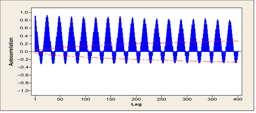
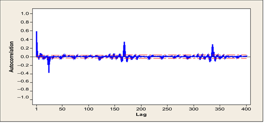
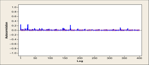
Figure 4 shows the estimated ACF after the daily and weekly seasonal differencing, which indicates that the series becomes stationary after eliminating the daily and weekly seasonal patterns. Lag polynomials up to order three are considered for the seasonal AR and moving average polynomials. Different DSARIMA models are estimated using maximum likelihood method. To estimate the parameters of the models and to check the forecasting performance, the whole year of 2017 hourly gas consumption is used as in-sample period to estimate DSARIMA models’ parameter, while the first month of 2018 hourly consumption put aside as out-of-sample period to evaluate the accuracy of the forecasts.
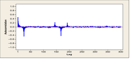
ACF of the Egyptian residential consumption after the daily and weekly differencing
ACF of the Egyptian residential consumption after the daily and weekly differencing
A Schwartz Bayesian criterion (SBC) is used to select a model from the different DSARIMA models. SBC is known as the Schwartz criterion and could be defined as:
where n is the sample data size, L ^ is the maximum likelihood estimate of the model and k is the number of parameters in the model. By choosing the model corresponding to the minimum value of SBC, one is selecting the model, that is, not over-fitted the data and has the highest probability (Schwarz, 1978). The SBC for the different orders of DSARIMA models are obtained. DSARIMA (3, 0, 2) (3, 1, 1)24(3, 1, 2)168 model is selected, as it has the lowest SBC.
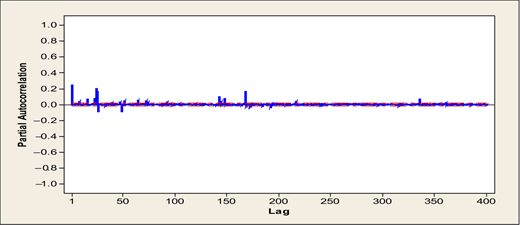
Secondly, to treat the volatility of the series, the squared residuals of the selected DSARIMA model are checked. Plotting the ACF and the partial ACF(PACF) of the squared residuals, as shown in Figures 5 and 6, confirmed the existence of GARCH effect. The PACF is similar to the ACF. It is also a tool to represent the statistical relationship between sets of ordered pairs of a time series.
Moreover, Table 1 summarizes the results of the Lagrange multiplier (LM) test to test the ARCHeffect. It clearly emphasizes on the presence of ARCH effect. The p-value is relatively small and less than the significance level 0.05. Hence, GARCH model is used in conjunction with DSARIMA to capture the volatility of the conditional variance.
LM test for heteroskedasticity
| Lag | Test statistic | p-value |
|---|---|---|
| 1 | 538.7906 | <0.0001 |
| 2 | 574.9881 | <0.0001 |
| 3 | 576.8938 | <0.0001 |
| 4 | 578.9294 | <0.0001 |
| 5 | 578.9402 | <0.0001 |
| 6 | 579.1947 | <0.0001 |
Lag order up to order two is often considered for GARCH models. Based on Schwartz criterion, DSARIMA (3, 0, 2) (3, 1, 1)24(3, 1, 2)168 + GARCH (1, 1) model yield the lowest SBC estimate among the different orders. The estimated results of this model are present in Table 2.
Estimated parameters for DSARIMA (3, 0, 2) (3, 1, 1)24(3, 1, 2)168-GARCH (1, 1) model
| Parameter | Estimate | Std. error | p-value |
|---|---|---|---|
| Φ1 | 1.5669 | 0.0431 | <0.0001 |
| Φ2 | −1.3317 | 0.0627 | <0.0001 |
| Φ3 | 0.4012 | 0.0285 | <0.0001 |
| Φ4 | 0.1612 | 0.0139 | <0.0001 |
| Φ5 | 0.1099 | 0.0127 | <0.0001 |
| Φ6 | 0.0654 | 0.0121 | <0.0001 |
| Ω1 | 0.6948 | 0.1156 | <0.0001 |
| Ω2 | −0.0136 | 0.0178 | 0.4448 |
| Ω3 | 0.0374 | 0.0156 | 0.0168 |
| θ1 | 1.0242 | 0.0394 | <0.0001 |
| θ2 | −0.8194 | 0.0396 | <0.0001 |
| Θ1 | 0.9009 | 0.0086 | <0.0001 |
| Ψ1 | 1.5165 | 0.1159 | <0.0001 |
| Ψ2 | −0.5406 | 0.1070 | <0.0001 |
| α1 | 0.0007 | 0.0030 | <0.0001 |
| α2 | 0.5140 | 0.0250 | <0.0001 |
| β1 | 0.2740 | 0.0203 | <0.0001 |
Hence, the estimated equations for the mean and the variance of the selected DSARIMA-GARCH model are
and
The MAPE is used then to check the accuracy of the forecasts produced by the identified model. The MAPE is calculated based on the difference between the actual and the forecasted values as follows:
(12)
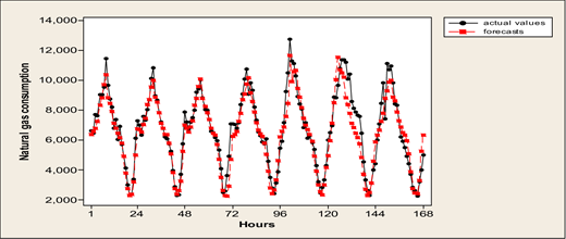
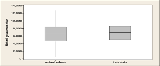
where yi and ŷi are the actual and the forecasted values respectively, while n is the number of forecasted values(Taylor, 2003; Taylor et al., 2006). The MAPE is calculated for 24 h-ahead, i.e. one day ahead, a week ahead and a month ahead. The percentages are 5.88%, 8.78% and 11.42% respectively. The MAPE for the different time periods are small. In addition, Figures 7 and 8 show how close the forecasts produced by the selected DSARIMA-GARCH model to the actual values of the Egyptian natural gas consumption series. This demonstrates the usage of DSARIMA-GARCH model that accommodates the volatile daily and weekly seasonal patterns of the Egyptian series in providing precision gas consumption forecasts to serve the energy power sector in Egypt.
6. Conclusion and future research
It is very important, for any country, to take into account the rapid increase of the natural gas consumption in their policies. Energy policymakers use forecasting methods as essential tools for adopting management policies. Providing an accurate forecasting of natural gas consumption for few hours ahead helps a lot in both maintaining and controlling the energy sector.
An important feature of the residential natural gas consumption series is the presence of both daily and weekly seasonal cycles. In this research, it is found, through the Egyptian residential gas consumption series, that the daily gas consumption has the same pattern every day. In addition, consumption, on weekends, is observed to be similar on different weeks but different compared to the other working days. Considering this feature can improve the accuracy of the forecasting.
Accordingly, DSARIMA-GARCH model is investigated in accommodating those daily and weekly seasonal patterns and capturing the volatility behavior of the Egyptian residential gas consumption series at the same time. Different orders of DSARIMA-GARCH models are estimated using maximum likelihood method. DARIMA-GARCH model with the lowest SBC is selected. The forecasts produced by the selected model are accurate for one day ahead, one week ahead and a month ahead. Hence, the selected model is recommended for forecasting the Egyptian residential natural gas consumption. It would be of a great importance for energy policymakers in Egypt.
For future research, DSARIMA-GARCH models could be used with different external variables such as temperature and weather variables. Further, different statistical approaches such as Bayesian approaches, could be investigated and compared with this approach in forecasting the Egyptian residential gas consumption.
