An M/M/C/K queueing system in an inventory routing problem considering congestion and response time for post-disaster humanitarian relief: a case study

Masoumi, Mahdieh; Aghsami, Amir; Alipour-Vaezi, Mohammad; Jolai, Fariborz; Esmailifar, Behdad

doi:10.1108/JHLSCM-12-2020-0119

Purpose

Due to the randomness and unpredictability of many disasters, it is essential to be prepared to face difficult conditions after a disaster to reduce human casualties and meet the needs of the people. After the disaster, one of the most essential measures is to deliver relief supplies to those affected by the disaster. Therefore, this paper aims to assign demand points to the warehouses as well as routing their related relief vehicles after a disaster considering convergence in the border warehouses.

Design/methodology/approach

This research proposes a multi-objective, multi-commodity and multi-period queueing-inventory-routing problem in which a queuing system has been applied to reduce the congestion in the borders of the affected zones. To show the validity of the proposed model, a small-size problem has been solved using exact methods. Moreover, to deal with the complexity of the problem, a metaheuristic algorithm has been utilized to solve the large dimensions of the problem. Finally, various sensitivity analyses have been performed to determine the effects of different parameters on the optimal response.

Findings

According to the results, the proposed model can optimize the objective functions simultaneously, in which decision-makers can determine their priority according to the condition by using the sensitivity analysis results.

Originality/value

The focus of the research is on delivering relief items to the affected people on time and at the lowest cost, in addition to preventing long queues at the entrances to the affected areas.

1. Introduction

Humans have been dealing with natural disasters at all times, and despite advances in technology over the past decades, they have never been able to prevent their occurrence. These disasters are constantly occurring and cause a lot of injuries in different areas. The rate of occurrence of natural disasters such as earthquakes and tsunamis has risen over time. Consequently, the number of victims due to socioeconomic-demographic factors, such as population growth and urban development, has increased (Hoeppe, 2016). Nevertheless, the number of people who lose their lives in these events is declining (The International Disaster Database, 2021). However, large earthquakes such as earthquakes in Turkey (İzmir, 1999), Taiwan (Chichi, 1999), India (Gujarat, 2001), Iran (Bam, 2003), Pakistan (Kashmir, 2004), China (Sichuan, 2008) and Haiti (Port-au-Prince, 2010) killed about 450,000 people. As a result, being prepared and aware of the appropriate disaster response is of considerable importance, which has attracted the attention of researchers in the field of disaster management (Barzinpour and Esmaeili, 2014).

Disaster management encompasses a wide range of activities related to before, during, and after natural and manmade disasters, including mitigation, preparation, response and recovery (Holguín-Veras et al., 2012). The mitigation phase involves long-term solutions to prevent disasters or reduce their effects. In the preparation phase, long-term decisions are made about the number and location of distribution sites so that the necessary measures can be taken with the least difficulty at the time of the accident. The response stage is the first step after the disaster, which is consists of operational decisions and all measures taken to attend to the affected people, including decisions about the route of vehicles, personnel and equipment. The last phase is the recovery stage that reconstructs the affected areas is its most crucial activity (Ahmadi et al., 2015).

Due to the severity of the accident and the damage caused in post-disaster conditions, the access of affected people to the essential items is limited, so using the appropriate distribution system will diminish human suffering as well as possible damages and losses. The focus of this article is on the response phase. This section is also called post-disaster humanitarian logistics, or PD-HL, which distributes essential goods such as water and food to the affected areas to decrease the aftermath of the disaster.

Depending on the type of problem, vehicle routing problem (VRP) techniques are utilized at this stage to solve the problem to deliver the relief products at the proper time and the right amount. Many factors challenge these problems, including disruption in delivering the goods to distribution centers, damages to relief routes, shortages in distribution centers, and so on. In classical VRP, the goal is to reduce total costs (Campbell et al., 1998). But in humanitarian arrangements, goals other than costs are also considered. Preliminary measures should be taken within the first 72 h after the disaster (Mitsotakis and Kassaras, 2010), so in humanitarian aid, the main focus is on relief response time. Since this study seeks to distribute goods to demand points after stabilizing conditions, the objective function is a combination of classical VRP goals and humanitarian logistics. In the process of distributing relief items, these commodities are transported from several distribution centers to the affected zones through designated routes. One of the logistics strategies to improve the performance and efficiency of the supply chain is to manage and control the inventory of border warehouses. This is because warehouse inventory directly impacts inventory holding costs, as well as the allocation of demand points to warehouses and, consequently, routing costs. Therefore, inventory control is one of the vital factors in determining the efficiency of the relief supply chain. It should be noted that border warehouses are warehouses that we select at the border of the affected areas to deliver relief aids that we receive from other areas. Due to the fact that it is usually practically impossible to enter the affected areas after a disaster occurrence, these warehouses are selected at the border of the affected areas. For example, in real-life rescue, planes or helicopters always deliver relief supplies to warehouses located on the border of affected areas.

According to the amount of humanitarian aid and the volume of goods that are sent to the warehouses in a short period, the queues' formation at the entrances of the border warehouses of the affected areas is inevitable.

On November 12, 2017, a destructive earthquake measuring 7.3 on the Richter scale jolted the province of Kermanshah in the western part of Iran. This was the strongest and deadliest earthquake of 2017, which took 630 lives, left more than 8,100 injured, and made 70,000 people homeless (Ahmadi and Bazargan-Hejazi, 2018). Unfortunately, mismanagement causes some problems such as congestion at the entrances of the city. This congestion caused the vehicles carrying relief items to wait in long queues for a long time in a crisis situation where people are waiting for these items. Also, the long queues that had formed had disrupted the possibility of relief in proper time and the arrival of relief vehicles. In contrast, proper management and determination of the appropriate number of warehouse servers could prevent such a situation. In critical situations after the catastrophe, people should not worry about the necessary items. Attempts should be made to minimize congestion at the entrances so that other relief activities can be carried out unhindered so that long queues of trucks and other arrival vehicles can disrupt by impeding the passage of relief vehicles. That's why we were motivated to develop a model to improve the distribution of materials between demand points by determining the optimal number of servers in border warehouses.

Moreover, to the best of our knowledge, designing a material distribution system considering the route congestion is not addressed at all in humanitarian logistic (HL) literature. As one of the operational performance criteria is service time level in the network, a mismatch between the arrival rate of flows and the processing rate of servers may cause congestion in the borders. After the disaster, aid will be sent to the affected areas by both the government and the people. Due to the limited capacity of unloading stations and the time-consuming process of unloading the vehicles, a queue will be formed when the number of vehicles is more than the number of servers, and here, due to the multiplicity of entrance vehicles and the limited number of servers after the disaster, a queue of vehicles will be formed that cause congestion. Timperio et al. (2017) also defined congestion as one of the eight important location criteria for site selection in a disaster relief network. Owing to the prolonging of these queues, the waiting time increases, and the rescue process will delay, which will have a severe impact on system performance. Long waiting times of vehicles in the queues while facing a lack of facilities and resources will increase the unemployment time of these vehicles, while at this time they can return and re-transport the goods to the affected areas, which can maximize productivity throughout the network and minimize wasted time. The result is more delivered goods to the affected areas in a shorter time. Prolonging the queues may cause the roads to be closed and disrupt the passage of relief vehicles, such as ambulances and firefighters. Traffic intensity represents the ratio of total demand to system capacity. The more servers establish, the shorter and less dense the queue will be, but the unemployment rate of the service mechanism will increase. Therefore, this article tries to balance all these performance measures by selecting and allocating the appropriate number of servers so that there is no high density in the system, no high unemployment service mechanism, and no long response time. Accordingly, applying the proposed method will lead to an efficient system.

In this article, we seek to reduce concerns about the delivery time of goods to the affected areas after the disaster. To achieve this purpose, we examined the response time to the demand points and the time that the vehicles may wait in the queues before the warehouses. By reducing the waiting time of the vehicles, the process of storing goods in the warehouses will be shortened, and vehicles will be more efficient by delivering more goods to more affected areas.

We divide the problem into three phases: Unloading relief items from vehicles, managing and controlling the warehouses' inventory and routing to distribute items between the demand points; in the first part, we are looking to shorten the waiting time for vehicles in the queues which is achieved by increasing the number of servers. It should be mentioned that servers in this article are the border warehouses. On the other hand, in the second phase, increasing the number of servers increases the filling rate of each warehouse and consequently increases warehousing costs. In this article, we seek to find the optimal number of servers by creating a balance between these two phases.

Eventually, in HL problems, the most substantial goal is to deliver items to different places promptly on time, which is the purpose of the third phase. In the presented model in this paper, by reducing the average weighted response time to the demand points, we seek to enhance the response level, and simultaneously, by decreasing transportation costs, we aim to augment efficiency.

VRP and inventory control are among the NP-hard problems, and combining these two types of issues with the queuing system will lead to more complexity. The separate optimal answers to these problems will not lead to an inclusive optimum result for the whole system, so it is vital to look for a comprehensive and optimal answer to the entire procedure. The main contribution of this study is to establish a correlation between productivity and system responsiveness. Accordingly, a bi-objective mixed-integer linear mathematical programming has been developed in this study to reduce the cost of routing and inventory storage and lessen the waiting time of vehicles to unload the items in warehouses and average weighted response time to the demand points. To achieve the above-mentioned objectives, the optimal number of servers as well as the best routes for distributing relief goods should be identified.

Thus, questions that should be addressed in this research are as follows:

RQ1.

How many servers should be allocated to each border warehouse for goods unloading to avoid long queues of vehicles and to minimize the average waiting time for vehicles?

RQ2.

To which warehouses should each of the demand points be allocated so that according to their inventory, they can be supplied without shortage?

RQ3.

What is the distribution route of the relief goods in the last phase of the problem in order to minimize the response time?

In order to answer the above questions, in this paper, a three-objective mathematical model has been developed to minimize the waiting time of vehicles and reduce congestion at the boundaries of the affected area to help minimize the response time to demand points and the total inventory holding costs. The objective of this paper is to calculate the optimal number of unloading servers, determine the appropriate allocation of demand points to border warehouses and specify the optimal route for goods distribution.

The remainder of this study is arranged as follows: The second section will address the literature review of the relief supply chain in addition to the inventory-routing models and the queue models in this field. In the third section, problem modeling and research methodologies are given. In section four, the exact and meta-heuristic methods to solve small and large-size problems are applied. The fifth section presents the results and numerical analysis of an example based on the 2017 Iran–Iraq earthquake. Finally, the conclusion is given in the sixth section of this study.

2. Literature review

In this section, the reviewed studies will first be proposed to show the literature gap and innovations of this study. Accordingly, research hypothesizes will be illuminated to put an end to this section.

2.1 Inventory-routing problem in disaster relief

The rising trend in the number of natural disasters and the increasing emphasis on accountability has been the motivating factors in enhancing humanitarian relief capacity and appropriate response. Also, many studies have been conducted in this field. Facility location models, relief distribution and transportation models, as well as multi-commodity network models generally bring about quantitative tools and optimization methods, which analyze the relief chain management, to optimize the flow of relief resources through the distribution networks.

Yi and Özdamar (2007) proposed an integrated location-routing model in the disaster response phase that coordinates the evacuation process and logistics support. Berkoune et al. (2012) presented a mathematical model for the transfer of relief goods to affected areas by minimizing the traveling time of distribution vehicles. They also proposed an efficient heuristic algorithm that can be used in realistic situations. Battini et al. (2014) developed a distribution model that concerns vehicle routing decisions and resource allocation. A model and algorithm of routing and dispatching have been developed by Najafi et al. (2014) in which distributing relief goods among the affected areas is focused in addition to transferring of injured people to hospitals. In this regard, the objective function of their proposed model includes minimizing the waiting time of injured people from the moment of the accident to the time of arrival at the hospital and also minimizing the waiting time of people from the moment of need to the arrival of relief items. Moreover, to ensure the efficiency and effectiveness of the response, it is possible to update the plan if the network changes. In this case, the items and people who may be on the routes are also taken into account. Sheu and Pan (2015) have presented a different random approach to dealing with the imbalance between demand and supply of essential products at the disaster condition. In this case, they have determined the demand in the affected zones using stochastic dynamic programming. Finally, they performed several numerical experiments to demonstrate the importance of relief suppliers in detracting the impacts of an unbalanced supply chain. Furthermore, Huang et al. (2015) provided a mathematical model consisting of three main objective functions of humanitarian logistics including lifesaving utility, delay cost, and fairness to optimize the response phase in the disaster situation. They also simulated the dynamic space of the problem with a time-space network and a rolling horizon approach so that the information about the time of the paths and the demand of the points is constantly updated. Camacho-Vallejo et al. (2015) have been studied humanitarian logistics at two levels. They have examined the aid distribution of international non-profit organizations and other countries after the disaster as a leader-follower game. These institutions (followers) seek to reduce transportation costs, while disaster-stricken countries (leaders) are looking to improve responsiveness and efficiency. Also, Rezaei-Malek et al. (2016) examined the pre-disaster phase to provide an integrated model for optimizing location-allocation and distribution. They also used the best order policy to restore perishable products. Smadi et al. (2018) presented research on delivering drinking water to affected people in the post-disaster phase of humanitarian logistics. An optimization method for the efficient distribution of post-disaster relief was presented by Vahdani et al. (2018). They proposed a two-phase multi-objective mixed-integer, multi-commodity, and multi-period mathematical modeling that examines three levels of the supply chain. In this model, decisions are made about the location of warehouses and their inventory management, as well as routing and distribution of relief items, according to the hard time window. Furthermore, this model has been developed to deal with uncertainty by using a robust optimization approach. They used NSGAII and MOPSO to solve large-size problems and evaluated the efficiency of the proposed algorithms via solving several instances. Tavana et al. (2018) have proposed a multi-level humanitarian logistics model in which the location of central warehouses and the number of perishable items that are related to the first phase of the article, have been examined. Moreover, the routing of goods from warehouses toward hospitals is identified as the article's second phase. A formulation has been developed by Chapman and Mitchell (2018) to choose the location of distribution centers from a list of candidate facilities. They used objective function terms to focus on fairness. Gökçe and Ercan (2019) have focused on pre-disaster activities. They have examined a new activity in Turkey called Neighborhood Disaster Stations, which includes containers holding items needed during a disaster that has been installed in specific locations (Alipour Vaezi and Tavakkoli-Moghaddam, 2020) proposed a new study about location-allocation of the COVID-19 (as a pandemic disaster) preparedness centers using multi-criteria decision making. They have examined the reliability of their research investigating a real-life case study. Abazari et al. (2020) developed a multi-objective Mixed-Integer Non-Linear programming to deliver relief items in addition to locating relief centers and determining their prepositioned inventory level. Danesh Alagheh Band et al. (2020) developed a multi-objective model to assess the conditions of roads and areas considering two types of assessment teams under uncertain parameters. Sakiani et al. (2020) studied a real-life post-disaster distribution and redistribution of the relief goods using a three-phase systematic method, which has been solved by a simulated annealing (SA) meta-heuristic algorithm. The routing problem of relief batches has been studied in the research of Ekici and Özener (2020). Their method is based on the interdependence of clustering techniques with inventory and routing allocation.

2.2 Application of the queueing theory in supply chain management and emergency condition

Unloading relief goods in warehouses is time-consuming, and due to the limited number of servers in the warehouses, vehicles ought to wait in the queues. The length of the queues is controlled by determining the appropriate number of servers. However, the observance of order and preventing congestion at the entrance warehouses are functionally important in providing relief to the affected areas, none of the reviewed studies have paid attention to the queues formed at the entrances of the warehouses. The congestion of vehicles at the borders causes a tough condition for emergency vehicles (ambulances, firefighters, etc.) to enter. Additionally, by shortening the waiting time for vehicles in the queues for unloading goods at border crossings, we can better use trucks in times of crisis when we face limited transport resources. Vehicles can be used to transport essential goods to the affected areas instead of spending a lot of time in long queues. In this section, valuable studies on queueing systems' application in supply chain management have been proposed.

Mohammadi et al. (2011) presented a mathematical model of hub covering location using the m/m/c queuing system, which aims to minimize transportation outlays in addition to fixed costs of hubs' establishment. An M/M/1 queueing system has been applied in a closed-loop supply chain network by Saeedi et al. (2015) in which the decision-maker should create a balance between costs and capacity of facilities. Zahiri et al. (2014) have proposed a bi-objective mathematical programming model of an organ transplant transportation network under uncertainty. The goal is to minimize transportation costs and time, such as waiting time in the queues for the transplant operation. Vass and Szabo (2015) presented a queuing model to reduce the waiting time in the Emergency Department (ED). Rahimi et al. (2016), have applied the M/M/C/K queue system in the hub network design with several objective functions considering the density created in the hubs. Ding et al. (2016) examined energy consumption and density simultaneously on a wireless sensor network. In the research of Aziziankohan et al. (2017), using queueing theory and transportation models, a new method for green supply chain management has been proposed to handle congestions and reduce energy consumption. Stojčić et al. (2018) developed an adaptive neuro-fuzzy inference system (ANFIS) model to optimize the queueing system in warehouses with two servers. They examined their method in a brown paper factory as a real-life case study. Ghodratnama et al. (2019), using queueing theory and fuzzy mathematical programming and by considering congestion in manufacturing plants, proposed a bi-objective mathematical model to address the production planning in industrial townships as a hub location-allocation problem. Mohtashami et al. (2020) examined a green closed-loop supply chain and included the G/M/s/M queueing system in their proposed model to reduce environmental impacts and energy consumption.

2.3 Research gaps

To the best of our knowledge, this is the first time that attention has been paid to the queue system in disaster literature. Through the presented model of this article, we purpose to fulfill the gaps in the literature as follows:

Representing a multi-objective inventory-routing model aims to reduce costs and decrease the waiting time of trucks and the average weighted response time to the affected areas.
Modeling the density at the entrance of the warehouses by calculating the waiting time of the trucks at the entry points of the depots and determining the optimal number of servers for each of the warehouses using the M/M/C/K queue model.
Using the M/M/C/K queue model for the vehicles at the entry points of the depots in an inventory-routing problem after the disaster.
Different vehicles at each border warehouse such as trucks, helicopters, and so on.

The presented paper will fill the mentioned gaps by proposing a three-objective mathematic model. Using this method, by determining the optimal number of servers in each warehouse and distribution routes besides defining the most efficient allocation of demand points to border warehouses, the waiting time of the vehicles, the response time to the demand points, and overall cost of inventory holding will be minimized.

2.4 Research hypotheses

The hypotheses that have been taken into consideration for modeling the proposed queuing-inventory-routing problem are as follows:

H1.

Raising the unloading rate reduces the waiting time of vehicles in the queue and thus lessens the number of vehicles in the queues. Moreover, as the rate of unloading items increases, it is possible to unload more vehicles. Thus, the increment in the number of items stored in warehouses and consequently escalating the cost of the system have resulted.

H2.

The more the number of servers in each warehouse, the better the response level to input vehicles. It also shortens the average waiting time for vehicles in the queue and reduces the length of queues formed at entry points. However, increasing the number of servers will raise the response rate to the vehicles. So, the inventory of the warehouses will grow faster, and more costs will be imposed on the system.

3. Problem description and formulation

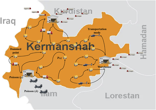
Generally, after the disaster and over the initial and emergency hours when the situation becomes steady, essential items should be regularly available to those affected by the disaster, owing to the resource's limitation in the affected areas. In this study, a multi-objective, multi-period, multi-item inventory-routing model is presented for distribution in post-disaster conditions to deliver items promptly and in the right amount. The relief network, which includes demand points and several main warehouses at border points, is shown in Figure 1. Each warehouse is dedicated to a specific mode of transportation such as trucks, helicopters, and so on. In a period, relief items collected by institutions and people are hauled from different cities to the border warehouses by various modes of transportation. Every vehicle needs an uncertain amount of time to unload its cargo. In situations where the number of vehicles is more than servers, a queue of vehicles is formed at each warehouse. Figure 1 also illustrates that the lack of a sufficient number of servers causes queues in the entry paths of the disaster area. According to a Poisson process, the vehicles arrive at the warehouse and vehicle unloading time follows the exponential distribution. There are some servers for unloading vehicles in each warehouse and waiting room capacity for vehicles is limited so in each warehouse, a multi-server Markovian queue with finite capacity will be formed. The model has tried to avoid congestion in the main roads and relief disruption, by optimizing the M/M/C/K queuing system in the border points.

Figure 1

View large Download slide

Structure of the distribution network and queues in border warehouses

The process of entering trucks into the system is a counting process in the form of ${N (t), t \geq 0}$ ⁠, in which the number of events at the start is zero (⁠ $N (0) = 0$ ⁠). Furthermore, since the number of events (truck entry) that occur in a given period is independent of the number of events that occur in another period that do not overlap, this process has the property of independent increments. For example, it is clear that the number of trucks that are entered between 8 and 9 a.m. is completely independent of the number of trucks that are entered between 10 and 11 a.m. Besides, the truck entry process also has stationary increments. That is, the number of trucks that enter the system at each time interval depends only on the length of the interval. Due to the fact that goods sent from different cities are not necessarily sent at a time and each truck may have moved from different cities at a particular time, so the number of trucks entered into the system depends only on the length of the interval and is independent of the time of their entrance. Given that these three properties are established; According to Ross (2014), it can be said that the process of entering trucks follows a Poisson process. On the other hand, according to the Poisson process's assumption, the intervals between trucks' entrances will follow an exponential distribution. Given that a disaster has occurred, it is more likely that these intervals will take a small amount than it will take large amounts because, with the occurrence of a disaster, people from all parts of the country try to deliver their goods to the affected area as soon as possible. So obviously, it is fully compatible with exponential distribution.

After completing the unloading process, these items are stored in warehouses and then transported to needing points of the disaster area using other vehicles according to the specified routes. In this research, by determining the number of servers for unloading the trucks, allocating demand points to warehouses, and also ascertaining distribution routes, we seek to enhance the level of responsiveness to injured people (reducing the average of the weighted response times), decrease transportation and inventory costs as well as lessen the waiting time for the trucks at the border points.

3.1 Assumptions

Each demand point in every period is allocated to only one warehouse, and also the demand of each zone is met by one vehicle, and we do not have split delivery.
After reaching the demand points, the vehicles unload the items on the site and then go to the next points. As a result, the time required to transport these items is a combination of the transportation time between points and unloading time.
The transportation time between the two points as well as the time of unloading the goods at the demand points, is considered deterministic.
If the waiting area of warehouses is full, vehicles will not be able to enter them.
The initial inventory of all warehouses is zero.
It is assumed that the distributed goods to demand points will be deducted from the inventory together in each period.

3.2 Notations

In the following, the equations for the developed mathematical model are described. Table 1 presents the used notations in the mathematical model.

Table 1

Table of notations

Sets
$V$	Set of indexes for warehouses $v \in V$
$T$	Set of indexes for periods $t \in T$
$I$	Set of indexes for demand points $i \in I$
$F$	Set of indexes for products $f \in F$
Parameters
$λ_{v t}$	The arrival rate of vehicles at the warehouse $v$ in the period $t$
$µ_{v t}$	Unloading rate at the warehouse $v$ at period $t$
$ρ_{v t}$	The traffic intensity of queue formed warehouse $v$ in the period $t$
$k_{v}$	Waiting rooms space for the warehouse $v$
$S_{v}$	Maximum number of servers at the warehouse $v$
${cap}_{v f}$	The capacity of arrival vehicles to the warehouse $v$ for product type f
$p_{i t f}$	The demand of demand point $i$ in the period t for product type f
$Q_{v f}$	The capacity of distribution vehicles of the warehouse $v$ for product type f
$τ_{i l}$	The traveling time between demand point $i$ and demand point $l$
$τ_{i v}^{'}$	The traveling time between demand point $i$ and warehouse $v$
$c_{i l}$	Traveling cost between demand point $i$ and $l$
$w t_{i}$	Importance of demand point $i$
$B_{i}$	Unloading time in the demand point $i$
$ω_{v f}$	Inventory cost of warehouse $v$ for product type $f$
Decision variables
$s_{v}$	Number of allocated servers to warehouse $v$
$w_{v t}$	Average waiting time for vehicles in the warehouse $v$ in the period $t$
$w q_{v t}$	Average waiting time for vehicles in the queues in the warehouse $v$ in the period $t$
$L_{v t}$	The average number of vehicles in the warehouse $v$ in the period $t$
$L q_{v t}$	The average number of vehicles in the queues in the warehouse $v$ in the period $t$
$π_{n}^{v t}$	Probability of existence of n vehicles in the warehouse v in the period t
$I_{v t f}$	Inventory level of product f in the warehouse v at the end of the period t
$z_{i v t}$	If demand point i is assigned to warehouse v in the period t 1, otherwise 0
$x_{0 i}^{v t}$	If demand point i is the first demand point in any route of warehouse v in the period t
$x_{i l}^{v t}$	If demand point i is visited just after demand point i in any route of warehouse v in the period t
$x_{i 0}^{v t}$	If demand point i is the last demand point in any route of warehouse v in the period t
$u_{t i f}$	A continuous variable which represents the load of the vehicle after visiting demand point i in the period t
$r_{i v t}$	Response time to the demand point i in the period t if it is allocated to the warehouse v

3.3 Modeling of vehicle queuing system

In this section, a model for queues of vehicles in the entrance of warehouses is described and the probabilities of steady-state, entry rate, length of the queues, and average waiting time of vehicles are calculated. The vehicles' entrance into warehouses follows the distribution of Poisson with the parameter of $λ_{v t}$ and in case of the existence of an empty server, vehicle unloading time follows the exponential distribution with an average of $\frac{1}{µ_{v t}}$ ⁠. The number of servers and the waiting space capacity of each warehouse are limited, so we will have an M/M/C/K queuing system.

We have used the following equations to model this queue system:

According to Ross (2014), the input and output rates are equal in queuing systems in a steady state. The entry rate of vehicles into warehouses is $λ_{v t}$ and in (⁠ $1 - π_{k}^{v t}$ ⁠) percent of times these vehicles can enter the queue to unload items, so the entry rate of vehicles in the queues in this system is calculated from Equation (1):

{\bar{λ}}_{v t} = λ_{v t} (1 - π_{k}^{v t}) \forall t, v

(1)

According to Shortle et al. (2018) the average waiting time in the warehouse is obtained from Equation (2):

w_{v t} = \frac{L_{v t}}{λ_{v t} (1 - π_{k}^{v t})} = w q_{v t} + \frac{1}{µ_{v t}} \forall t, v

(2)

On the other hand, the average waiting time in the queue can be calculated from Equation (3):

w q_{v t} = \frac{L q_{v t}}{λ_{v t} (1 - π_{k}^{v t})} \forall t, v

(3)

And the idle probability of servers for unloading the vehicles in the warehouses can be obtained from equation (4):

π_{0}^{v t} = {\begin{matrix} {\sum_{n = 0}^{s_{v} - 1} {(\frac{λ_{v t}}{µ_{v t}})}^{n} \frac{1}{n!} + \frac{{(\frac{λ_{v t}}{µ_{v t}})}^{s_{v}}}{s_{v}!} (k_{v} - s_{v} + 1)}^{- 1} & ρ_{v t} = 1 \\ {\sum_{n = 0}^{s_{v} - 1} {(\frac{λ_{v t}}{µ_{v t}})}^{n} \frac{1}{n!} + \frac{{(\frac{λ_{v t}}{µ_{v t}})}^{s_{v}}}{s_{v}!} \frac{1 - ρ_{v t}^{k_{v} - s_{v} + 1}}{1 - ρ_{v t}}}^{- 1} & ρ_{v t} \neq 1 \end{matrix} \forall t, v

(4)

Equation (5) calculates the probability of existing n vehicles in the warehouse v:

π_{n}^{v t} = {\begin{matrix} \frac{1}{n!} {(\frac{λ_{v t}}{µ_{v t}})}^{n} π_{0}^{v t} & 0 \leq n \leq s_{v} \\ \frac{1}{s_{v}!} \frac{1}{s_{v}^{n - s_{v}}} {(\frac{λ_{v t}}{µ_{v t}})}^{n} π_{0}^{v t} & s_{v} \leq n \leq k_{v} \end{matrix} \forall t, v

(5)

Using equation (5) the average number of vehicles in the system and the average number of vehicles in the queue in every warehouse can be obtained from equation (6) and (7), respectively:

L_{v t} = L_{q} + c - π_{0} \sum_{n = 0}^{c - 1} (c - n) \frac{{(\frac{λ}{µ})}^{n}}{n!} \forall t, v

(6)

L q_{v t} = \frac{π_{0}^{v t}}{s_{v}!} {(\frac{λ_{v t}}{µ_{v t}})}^{s_{v}} \frac{ρ_{v t}}{{(1 - ρ_{v t})}^{2}} {1 - ρ_{v t}^{k_{v} - s_{v} + 1} - (1 - ρ_{v t}) (k_{v} - s_{v} + 1) ρ_{v t}^{k_{v} - s_{v}}} \forall t, v

(7)

And the traffic intensity of queue formed in every warehouse can be obtained from equations (8):

ρ_{v t} = \frac{λ_{v t}}{s_{v} µ_{v t}} \forall t, v

(8)

Finally, constraint (9) specifies the maximum number of servers allowed per warehouse:

s_{v} \leq S_{v}

(9)

3.4 Inventory model of border warehouses

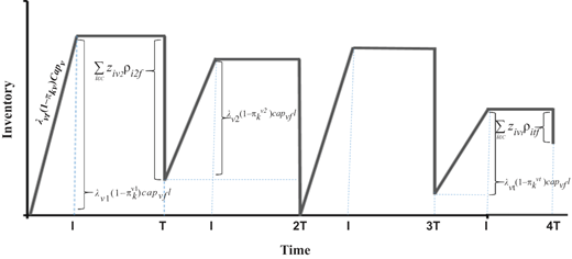
This study assumes that vehicles distribute the items stored in warehouses between demand points at the beginning of each period. Therefore, the inventory level at the beginning of each period is calculated according to the inventory level in the previous period. Figure 2 demonstrates the inventory changes over time. T represents the cycle time in this figure, and l is the period when items enter the warehouses (l < T). As mentioned in section 3.3, the entry rate of vehicles in the queue in this system will be equal to $λ_{v} (1 - π_{k v})$ ⁠. If the capacity of each device is ${Cap}_{v}$ ⁠, then the filling rate of the warehouses at each period will be equal to $λ_{v t} (1 - π_{k v}) {Cap}_{v}$ ⁠.

Figure 2

View large Download slide

Inventory level over time

As mentioned, the essential items are distributed between the demand points at the beginning of each period. Therefore, at the starting point of each period, the inventory of the warehouses decreases as much as the total demand of demand points assigned to them, and it is obtained from the following relationships:

\begin{array}{l} I_{v 1 f} = λ_{v 1} (1 - π_{k}^{v 1}) {cap}_{v f} l \forall v, f \\ I_{v 2 f} = I_{v 1 f} - \sum_{i \in C} z_{i v 2} p_{i 2 f} + λ_{v 2} (1 - π_{k}^{v 2}) {cap}_{v f} l \forall v, f \\ I_{v 3 f} = I_{v 2} - \sum_{i \in C} z_{i v 3} p_{i 3 f} + λ_{v 3} (1 - π_{k}^{v 3}) {cap}_{v f} l \forall v, f \end{array}

(10)

⋮

I_{v t f} = I_{v (t - 1) f} - \sum_{i \in C} z_{i v t} p_{i t f} + λ_{v t} (1 - π_{k}^{v t}) {cap}_{v f} l \forall t, v, f

(11)

The proposed model is related to post-disaster conditions, and due to the urgency of the situation, planning should be such that we do not face shortages. As a result, constraint (12) prevents the shortage of inventory:

I_{v (t - 1) f} - \sum_{i \in C} z_{i v t} p_{i t f} \geq 0

(12)

Inventory holding cost is one of the main costs that crisis managers face in disaster management. The total inventory holding cost is obtained as depicted in equation (13) by multiplying the cost of holding one unit per time by average inventory maintained per time, whereas average inventory maintained per time is calculated from the area below Figure 2. In this figure, it can be seen that in each time period T, a trapezoid and a rectangle can be drawn below the inventory diagram, and the area of all of them can be added to calculate the area under the inventory diagram. Given that there is no initial inventory in the first period, there is only one trapezoid and the area of the rectangle is zero. The area of the trapezoid can be calculated as $\frac{1}{2} (T + (T - l)) λ_{v 1} (1 - π_{k}^{v 1}) {cap}_{v f} l = (T - \frac{l}{2}) λ_{v 1} (1 - π_{k}^{v 1}) {cap}_{v f} l$ ⁠. Accordingly, for the second period, the area of the formed trapezoid can be calculated as $\frac{1}{2} (T + (T - l)) λ_{v 2} (1 - π_{k}^{v 2}) {cap}_{v f} l = (T - \frac{l}{2}) λ_{v 2} (1 - π_{k}^{v 2}) {cap}_{v f} l$ ⁠, and the formed rectangle will be equal to $T (I_{v 1 f} - \sum_{i \in C} z_{i v 2} p_{i 2 f})$ ⁠. If the total inventory is equal to the demand, obviously, the rectangle is omitted, and its area is calculated as zero. In the same way, for period $t$ ⁠, the area of a rectangle and a trapezoid can be calculated as $T (I_{v (t - 1) f} - \sum_{i \in C} z_{i v t} p_{i t f})$ ⁠, $\frac{1}{2} (T + (T - l)) λ_{v t} (1 - π_{k}^{v t}) {cap}_{v f} l = (T - \frac{l}{2}) λ_{v t} (1 - π_{k}^{v t}) {cap}_{v f} l$ respectively. As a result, the sum of all rectangles and trapezoids from the beginning to the end of the time horizon is calculated from equation (13).

\sum_{f \in F} \sum_{v \in V} \sum_{t \in T} ω_{v f} (T - \frac{l}{2}) λ_{v t} (1 - π_{k}^{v t}) {cap}_{v f} l + \sum_{f \in F} \sum_{v \in V} \sum_{t \in T \neq 1} ω_{v f} T (I_{v (t - 1) f} - \sum_{i \in C} z_{i v t} p_{i t f})

(13)

3.5 Mixed-integer-nonlinear programming model

In this section, a new mathematical model for the inventory-routing problem has been developed by optimizing the inventory problem described in Section 3.4 and the queuing system described in Section 3.3. In the following, the equations for the developed mathematical model are described.

\min f 1 = \sum_{f \in F} \sum_{v \in V} \sum_{t \in T} ω_{v f} (T - \frac{l}{2}) λ_{v t} (1 - π_{k}^{v t}) {cap}_{v f} l + \sum_{f \in F} \sum_{v \in V} \sum_{t \in T \neq 1} ω_{v f} T (I_{v (t - 1) f} - \sum_{i \in C} z_{i v t} p_{i t f}) + \sum_{v \in V} \sum_{i \in I} \sum_{t \in T} (c_{v i} x_{0 i}^{v t} + c_{i v} x_{i 0}^{v t}) + \sum_{v \in V} \sum_{i \in I} \sum_{\begin{array}{l} l \in I \\ i \neq l \end{array}} \sum_{t \in T} c_{i l} x_{i l}^{v t}

(14)

\min f 2 = \sum_{i \in I} \sum_{v \in V} \sum_{t \in T} r_{i v t} w t_{i}

(15)

\min f 3 = \sum_{v \in V} \sum_{t \in T} w q_{v t}

(16)

s.t.

Eqs. (1)–(12)

\sum_{v \in V} z_{i v t} = 1 \forall i, t

(17)

\sum_{i \in I} x_{0 i}^{v t} = \sum_{i \in I} x_{i 0}^{v t} \forall v, t

(18)

\sum_{\begin{array}{l} i \in I \cup {0} \\ l \neq i \end{array}} x_{i l}^{v t} = z_{l v t} \forall v, l, t

(19)

\sum_{\begin{array}{l} l \in I \cup {0} \\ i \in l \end{array}} x_{i l}^{v t} = z_{i v t} \forall v, i, t

(20)

u_{t i f} - u_{t l f} + \sum_{v \in V} Q_{v f} x_{i l}^{v t} \leq \sum_{v \in V} Q_{v f} z_{i v t} - p_{t l f} \forall i, l, t, f | i \neq l

(21)

p_{t i f} \leq u_{t i f} \leq \sum_{v \in V} Q_{v f} z_{i v t} \forall i, t, f

(22)

r_{l v t} = (τ_{l v}^{'}) x_{0 l}^{v t} + \sum_{i} (r_{i v t} + B_{i} + τ_{i l}) x_{i l}^{v t} \forall v, l, t

(23)

u_{t i f}, r_{i v t}, I_{v t f} \geq 0 \forall v, i, t, f

(24)

z_{i v t}, x_{0 i}^{v t}, x_{i 0}^{v t}, x_{i l}^{v t} \in {0, 1} \forall v, i, l, t

(25)

π_{k}^{v t} \in [0, 1] \forall v, t, k

(26)

The proposed model includes 3 objective functions; the goal of the first objective function is to minimize the total economic costs, which include the two operating costs and holding costs of the average inventory transported from warehouses to demand points. The second objective function tries to reduce the average weight of the response time to the demand points. Finally, the purpose of the third objective function is to lessen the waiting time of the vehicles in the queues entering the warehouses. Constraint (17) ensures that each demand point is allocated to only one warehouse at a period. Constraint (18) equates the number of vehicles leaving warehouses with the number of vehicles returning to warehouses after distributing. Before and after each demand point, only one demand point or a warehouse should be designated in each route. Also, each demand point must be located along the route of the assigned warehouse. Constraints (19) and (20) apply to these cases, respectively. Constraints (21) and (22) have been created to prevent sub-tours. This Constraint is taken from the traveling salesman problem (Miller et al., 1960). The delivery time of relief items to the demand points includes the time of transport between the points and the time of unloading the cargo, which is defined in Constraint (23). Finally, the Constraints (24–26) specify the type of decision variables.

4. Solution methods

The model presented in this study is a multi-objective model with conflicting objective functions, as a result, to solve this model, the LP metric method is used, which reformulates the model into a single objective model. To solve the small-size examples of the model, an exact method named generalized algebraic modelling system (GAMS) is applied. However, due to the NP-hardness of the problem and time-consuming solutions of the precise methods, metaheuristic methods have been used to solve large-size problems. The grasshopper optimization algorithm is used to solve the presented model in this study. Eventually, to prove the validity and efficiency of the proposed algorithm, the results of small problem solving by the exact method and the results of the GOA algorithm are compared.

4.1 Multi-objective approach

Since the model presented in this study is a multi-objective problem, the LP-metric method, a multicriteria decision-making (MCDM) methodology to solve multi-objective models, has been utilized to convert this model into a single-objective one. This methodology is a rigorous multi-objective technique that makes a combined dimensionless objective by decreasing the relative deviations of the objective functions from their optimal value (Aryanezhad et al., 2009). This method has been applied in many studies such as Mohtashami et al. (2019, 2020), Mohammed and Wang (2017), Mirzapour Al-E-Hashem et al. (2011) and Rabbani et al. (2018). In this method, we define the new objective function as presented in equation (27).

Min f = \sum_{i = 1}^{k} γ_{i} {(- 1)}^{p} (\frac{f_{i}^{*} - f_{i}}{f_{i}^{*}})

(27)

Accordingly, $f_{i}^{*}$ is the optimal value of the objective function $i$ ⁠, and P equals to 2 for the functions to be maximized and 1 for the functions to be minimized. Also $γ_{i} \geq 0$ ⁠, which represents the weight of the target functions, must be true of the equation $\sum_{i} γ_{i} = 1$ and these values are determined by the decision-maker.

4.2 Grasshopper optimization algorithm

Saremi et al. (2017) proposed a meta-heuristic algorithm based on the grasshopper swarm intelligence, named Grasshopper optimization algorithm (GOA), to optimize challenging and time-consuming problems. GOA tries to find optimal solutions by mimicking and modeling the grasshopper swarm's behavior in nature and their group movement in search of food sources. This algorithm presents competitive results compared to other algorithms in the literature and it has been proven that it has efficient results for real problems with unspecified search spaces (Mirjalili et al., 2018). Logically, the search process is divided into exploration and exploitation proclivities by nature-inspired algorithms that grasshopper's life has these properties, naturally (Momeni et al., 2019). This is the essence of GOA which is represented in equation (28).

X_{i} = S_{i} + G_{i} + A_{i}

(28)

In equation (28), which illustrates the behavior of the grasshoppers, $X_{i}$ indicates the $i$ th grasshopper. Also, $S_{i}$ represents the social interaction, $G_{i}$ refers to the gravity force on the $i$ th grasshopper, and $A_{i}$ shows the wind advection. $S_{i} . G_{i} . and A_{i}$ obtain using equation (29), (33), and (34) respectively.

S_{i} = \sum_{j = 1}^{N} s (d_{i j}) \hat{d_{i j}} j \neq i

(29)

d_{i j} = | x_{j} - x_{i} |

(30)

\hat{d_{i j}} = \frac{x_{j} - x_{i}}{d_{i j}}

(31)

While equation (30) calculates the distance between the $i$ th and the $j$ th grasshopper, equation (31) computes the unit vector from the $i$ th grasshopper to the $j$ th grasshopper. Furthermore, the strength of the social forces in represent by $s$ function showed in equation (32).

s (r) = f e^{\frac{- r}{l}} - e^{- r}

(32)

Equations (33–35) calculates the parameters used in equation (28) using $g$ which indicates the gravitational constant, $\hat{e_{g}}$ which represents the unity vector towards the center of the Earth, $\hat{e_{w}}$ that is a unity vector in the direction of the wind, and $u$ is the constant drift.

G_{i} = - g \hat{e_{g}}

(33)

A_{i} = u \hat{e_{w}}

(34)

X_{i} = \sum_{j = 1}^{N} s (| x_{j} - x_{i} |) \frac{x_{j} - x_{i}}{d_{i j}} - g \hat{e_{g}} + u \hat{e_{w}} j \neq i

(35)

Based on $u b_{d}$ ⁠, $l b_{d}$ ⁠, and $\hat{T_{d}}$ which are respectively showing the upper bound, the lower bound, and the value of the $d$ th dimension, equation (36) has proposed to solve the problem. For better understanding it can be said that $\hat{T_{d}}$ indicates the best solution yet.

X_{i}^{d} = c (\sum_{j = 1}^{N} c \frac{u b_{d} - l b_{d}}{2} s (| x_{j}^{d} - x_{i}^{d} |) \frac{x_{j} - x_{i}}{d_{i j}}) + \hat{T_{d}} j \neq i

(36)

Due to the fact that the propeller algorithm is used for continuous space, in discrete cases, the initial answers must be generated continuously so that the exploration and extraction operate properly (Rajput et al., 2017; Abualigah and Diabat, 2020; Abazari et al., 2020). Then a discrete to continuous conversion must be performed. For example, to generate an answer grasshopper) that represents the number of servers in gate $v$ ⁠, a continuous vector for the gate has to be generated that the output value of each component is between 1 and $k_{v}$ (note that In a capacity queue system, the number of servers is at most equal to the amount of capacity). In that case, the GOA operators can perform exploration and extraction for this vector. Then, for the server number to be an integer and be used in calculating the objective function and other values, this vector must be rendered to become an integer. Other problem variables were generated and applied with the same approach.

5. Numerical example

5.1 Computational experiment

The model presented in this study is coded in GAMS 24.2.3. To prove the model's validity, small-scale solutions have been solved using the computer with core i7 CPU, 2.60 GHz, and 8 GB of RAM with BARON solver. But it takes a long time to solve large-scale examples using exact methods, and sometimes it can even take days. Therefore, heuristic and metaheuristic methods are commonly used to solve large problems. In this study, the GOA algorithm has been utilized to optimize the non-linear inventory routing. Finally, to prove the efficiency of the metaheuristic algorithm, the results of the small-size instance obtained from this algorithm are compared with the results acquired from the exact methods.

The parameters used for the small and large instances, are shown in Tables A1 and A2 respectively. Also, it has to be mentioned the information of the large numerical example is obtained by increasing the demand of demand points, the number of warehouses, the number of goods, and the number of time intervals of the small problem.

Table A1

Value of parameters for small-scale problem

Parameters	Value	Parameters	Value	Parameters	Value
$l$	8	${cap}_{11}$	60	$µ_{11}$	1.5
$T$	24	${cap}_{12}$	50	$µ_{12}$	1.65
$A_{1}$	0.2	${cap}_{21}$	80	$µ_{13}$	1.8
$A_{2}$	0.5	${cap}_{22}$	30	$µ_{21}$	2.25
$A_{3}$	0.3	$ω_{11}$	20	$µ_{22}$	1.05
$K_{1}$	7	$ω_{12}$	10	$µ_{23}$	1.5
$K_{2}$	8	$ω_{21}$	20	$τ_{12}$	2
$S_{1}$	5	$ω_{22}$	15	$τ_{13}$	2
$S_{2}$	6	$c_{12}$	1.5	$τ_{14}$	1
$B_{1}$	1	$c_{13}$	1.5	$\dots$	…
$B_{2}$	1	$c_{14}$	1.5	$τ_{54}$	4
$B_{3}$	1	$c_{15}$	2.2	$p_{111}$	8
$B_{4}$	1	$c_{21}$	2.5	$p_{112}$	6
$B_{5}$	1	$c_{23}$	1.9	$p_{211}$	20
$w t_{1}$	0.1	$c_{24}$	0.6	$p_{212}$	15
$w t_{2}$	0.2	$\dots$	…	$p_{311}$	20
$w t_{3}$	0.3	$c_{54}$	1.8	$p_{312}$	16
$w t_{4}$	0.2	$λ_{11}$	1	$p_{411}$	8
$w t_{5}$	0.2	$λ_{12}$	1.1	$p_{412}$	5
$Q_{11}$	50	$λ_{13}$	1.2	$p_{511}$	20
$Q_{12}$	50	$λ_{21}$	1.5	$\dots$	…
$Q_{21}$	50	$λ_{22}$	0.7	$p_{531}$	22
$Q_{22}$	50	$λ_{23}$	1	$p_{532}$	18

Table A2

Source of random generation of the parameters of large-scale example

Parameters	Value	Parameters	Value
$I$	70	$B_{v}$	[1,100]
$V$	15	$w t_{i}$	[0,1]
$F$	30	$Q_{v f}$	50
$T$	15	${cap}_{v f}$	[1,100]
$l$	8	$ω_{v f}$	[1,100]
$T$	24	$c_{i j}$	[1,50]
$A_{1}$	0.4	$λ_{v t}$	[1,50]
$A_{2}$	0.3	$µ_{v t}$	[1,50]
$A_{3}$	0.3	$τ_{i j}$	[1,100]
$K_{v}$	[5,15]	$p_{i t f}$	[1,200]
$S_{v}$	[5,15]

5.2 Parameters tuning

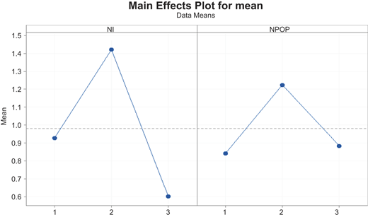
To achieve high-quality solutions by meta-heuristic algorithms, it is necessary to set the parameter correctly. In this section, using the Taguchi method, the parameters of the proposed algorithm have been set up. In this case, two GOA parameters, population size (N POP) and the number of iterations (NI) are selected as control factors in three levels. Table 2 shows these parameters and the levels of each parameter.

Table 2

Different levels of control factors

Level	NPOP	NI
1	40	25
2	60	50
3	80	100

First, nine different test problems are presented in Table 3 for different sizes. Then, related percentage deviation (RPD) of these test problems are computed through equation (37), by solving them thrice:

RDP = \frac{Z_{MH} - LB}{LB}

(37)

which, $LB$ is the lower bound of the objective function obtained by CPLEX solver after one hour and $Z_{MH}$ is the best value of the objective function by GOA. Finally, since the proposed model is multi-objective, the average of RPD is calculated for each experiment.

Table 3

Normalized results of Taguchi experiment

Run	Z1	Z2	Z3	RPD of Z1	RPD of Z2	RPD of Z3	$\bar{RPD}$
1	4.47*10⁶	110.88	1.43	0.15	0.26	3.08	1.16
2	4.16*10⁶	131.79	1.74	0.07	0.49	3.97	1.51
3	4.57*10⁶	129.53	1.8	0.18	0.47	4.1	1.59
4	4.47*10⁶	107	0.47	0.15	0.21	0.34	0.23
5	4.51*10⁶	94	2.35	0.16	0.06	3.71	1.98
6	3.95*10⁶	116.21	0.83	0.02	0.31	1.37	0.57
7	4.5*10⁶	108.55	1.4	0.16	0.22	3	1.13
8	4.21*10⁶	106.82	0.44	0.08	0.20	0.25	0.18
9	4.45*10⁶	96.03	0.79	0.14	0.09	1.25	0.49

Run	Z1	Z2	Z3	RPD of Z1	RPD of Z2	RPD of Z3	$\bar{RPD}$
1	4.47*10⁶	110.88	1.43	0.15	0.26	3.08	1.16
2	4.16*10⁶	131.79	1.74	0.07	0.49	3.97	1.51
3	4.57*10⁶	129.53	1.8	0.18	0.47	4.1	1.59
4	4.47*10⁶	107	0.47	0.15	0.21	0.34	0.23
5	4.51*10⁶	94	2.35	0.16	0.06	3.71	1.98
6	3.95*10⁶	116.21	0.83	0.02	0.31	1.37	0.57
7	4.5*10⁶	108.55	1.4	0.16	0.22	3	1.13
8	4.21*10⁶	106.82	0.44	0.08	0.20	0.25	0.18
9	4.45*10⁶	96.03	0.79	0.14	0.09	1.25	0.49

In the Taguchi method, Signal-to-Noise (S/N) criterion is a robustness measure that can be used to recognize the values of control factors that reduce variability by minimizing the effects of noise factors. “Smaller is better” type of S/N ratio can be used for objectives aimed to minimize the response which is computed by $- 10 * \log_{10} \frac{1}{n} {rpd}_{i}^{2}$ formula. This way, Figure 3 shows the values of the S/N ratio of each control factor in each level that NPOP and NI are set to 40 and 100, respectively.

Figure 3

View large Download slide

S/N ratio (smaller the better)

5.3 Model validation

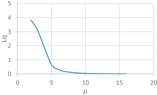
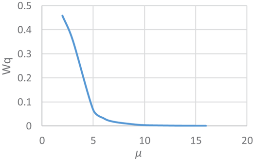
In this subsection, to guarantee the validity of the model and its reliability, sensitivity analysis on item unloading rate in warehouses (⁠ $µ_{v t}$ ⁠) has been performed to demonstrate its effect on the average length of queues as well as the waiting time of queuing vehicles. Obviously, as the unloading rate enhances, the length of the queues decreases, and consequently, the waiting time for vehicles in the queue becomes shorter. The diagram shown in Figures 4 and 5 indicates the sensitivity analysis results on this parameter. According to the obtained diagram, it is clear that with the increment in the discharge rate, the density at the entrance points of the warehouses decreases.

Figure 4

View large Download slide

Length of queue vs unloading rate

Figure 5

View large Download slide

Waiting time vs unloading rate

6. Results and discussion

6.1 Results

6.1.1 Small-scale problem

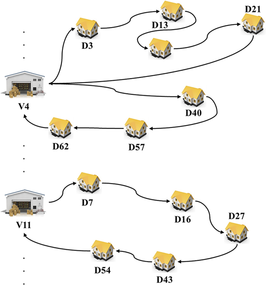
In this section, the optimal results of solving a small-scale problem (The information has been proposed in Appendix, Table A1) using the proposed model and GAMS software are obtained and shown in Table 4. Also, the path allocated to all warehouses in the first period is given in Figure 6. The value of the first, second, and third objective functions of solving this example is 4060415.110, 2.3, and 0.203, respectively. Moreover, the number of optimal servers for the first warehouse is 3, and it is 2 for the second distribution center. Note that these answers are obtained for setting the values of $γ_{i}$ as $γ_{1} = 0.2$ ⁠, $γ_{2} = 0.5$ and $γ_{3} = 0.3$ ⁠.

Table 4

The optimal solution for small size example by the exact method

The average waiting time in the system		The average waiting time in the queue		The average number of vehicles in the system		The average number of vehicles in the queue		Probability of existence of 0 vehicles in the system
$w_{11}$	0.667	$w q_{11}$	0.0090	$L_{11}$	0.674	$L q_{11}$	0.0098	$π_{0}^{11}$	0.510
$w_{12}$	0.606	$w q_{12}$	0.0071	$L_{12}$	0.674	$L q_{12}$	0.0098	$π_{0}^{21}$	0.492
$w_{13}$	0.556	$w q_{13}$	0.0064	$L_{13}$	0.674	$L q_{13}$	0.0098	$π_{0}^{12}$	0.510
$w_{21}$	0.489	$w q_{21}$	0.0040	$L_{21}$	0.741	$L q_{21}$	0.0801	$π_{0}^{22}$	0.482
$w_{22}$	1.028	$w q_{22}$	0.1135	$L_{22}$	0.726	$L q_{22}$	0.0599	$π_{0}^{13}$	0.511
$w_{23}$	0.728	$w q_{23}$	0.0632	$L_{23}$	0.735	$L q_{23}$	0.0720	$π_{0}^{23}$	0.488

The average waiting time in the system		The average waiting time in the queue		The average number of vehicles in the system		The average number of vehicles in the queue		Probability of existence of 0 vehicles in the system
$w_{11}$	0.667	$w q_{11}$	0.0090	$L_{11}$	0.674	$L q_{11}$	0.0098	$π_{0}^{11}$	0.510
$w_{12}$	0.606	$w q_{12}$	0.0071	$L_{12}$	0.674	$L q_{12}$	0.0098	$π_{0}^{21}$	0.492
$w_{13}$	0.556	$w q_{13}$	0.0064	$L_{13}$	0.674	$L q_{13}$	0.0098	$π_{0}^{12}$	0.510
$w_{21}$	0.489	$w q_{21}$	0.0040	$L_{21}$	0.741	$L q_{21}$	0.0801	$π_{0}^{22}$	0.482
$w_{22}$	1.028	$w q_{22}$	0.1135	$L_{22}$	0.726	$L q_{22}$	0.0599	$π_{0}^{13}$	0.511
$w_{23}$	0.728	$w q_{23}$	0.0632	$L_{23}$	0.735	$L q_{23}$	0.0720	$π_{0}^{23}$	0.488

Probability of existence of n vehicles		Probability of existence of n vehicles		Probability of existence of n vehicles		Response time
$π_{1}^{11}$	0.340	$π_{3}^{21}$	0.037	$π_{6}^{11}$	2.0805* $10^{- 4}$	$r_{121}$	4
$π_{1}^{12}$	0.340	$π_{3}^{22}$	0.036	$π_{6}^{12}$	2.0806* $10^{- 4}$	$r_{122}$	1
$π_{1}^{13}$	0.340	$π_{3}^{23}$	0.037	$π_{6}^{13}$	2.0807* $10^{- 4}$	$r_{123}$	1
$π_{1}^{21}$	0.328	$π_{4}^{11}$	0.006	$π_{6}^{21}$	0.001	$r_{221}$	2
$π_{1}^{22}$	0.322	$π_{4}^{12}$	0.006	$π_{6}^{22}$	0.001	$r_{222}$	2
$π_{1}^{23}$	0.325	$π_{4}^{13}$	0.006	$π_{6}^{23}$	0.001	$r_{223}$	2
$π_{2}^{11}$	0.113	$π_{4}^{21}$	0.012	$π_{7}^{11}$	6.2381* $10^{- 5}$	$r_{311}$	3
$π_{2}^{12}$	0.113	$π_{4}^{22}$	0.012	$π_{7}^{12}$	6.2405* $10^{- 5}$	$r_{312}$	4
$π_{2}^{13}$	0.113	$π_{4}^{23}$	0.012	$π_{7}^{13}$	6.2425* $10^{- 5}$	$r_{313}$	4
$π_{2}^{21}$	0.109	$π_{5}^{11}$	0.001	$π_{7}^{21}$	4.6109* $10^{- 4}$	$r_{411}$	2
$π_{2}^{22}$	0.107	$π_{5}^{12}$	0.001	$π_{7}^{22}$	4.5216* $10^{- 4}$	$r_{412}$	2
$π_{2}^{23}$	0.108	$π_{5}^{13}$	0.001	$π_{7}^{23}$	4.5735* $10^{- 4}$	$r_{413}$	2
$π_{3}^{11}$	0.025	$π_{5}^{21}$	0.004	$π_{8}^{21}$	1.5374* $10^{- 4}$	$r_{511}$	1
$π_{3}^{12}$	0.025	$π_{5}^{22}$	0.004	$π_{8}^{22}$	1.5076* $10^{- 4}$	$r_{512}$	1
$π_{3}^{13}$	0.025	$π_{5}^{23}$	0.004	$π_{8}^{23}$	1.5249* $10^{- 4}$	$r_{513}$	1

Probability of existence of n vehicles		Probability of existence of n vehicles		Probability of existence of n vehicles		Response time
$π_{1}^{11}$	0.340	$π_{3}^{21}$	0.037	$π_{6}^{11}$	2.0805* $10^{- 4}$	$r_{121}$	4
$π_{1}^{12}$	0.340	$π_{3}^{22}$	0.036	$π_{6}^{12}$	2.0806* $10^{- 4}$	$r_{122}$	1
$π_{1}^{13}$	0.340	$π_{3}^{23}$	0.037	$π_{6}^{13}$	2.0807* $10^{- 4}$	$r_{123}$	1
$π_{1}^{21}$	0.328	$π_{4}^{11}$	0.006	$π_{6}^{21}$	0.001	$r_{221}$	2
$π_{1}^{22}$	0.322	$π_{4}^{12}$	0.006	$π_{6}^{22}$	0.001	$r_{222}$	2
$π_{1}^{23}$	0.325	$π_{4}^{13}$	0.006	$π_{6}^{23}$	0.001	$r_{223}$	2
$π_{2}^{11}$	0.113	$π_{4}^{21}$	0.012	$π_{7}^{11}$	6.2381* $10^{- 5}$	$r_{311}$	3
$π_{2}^{12}$	0.113	$π_{4}^{22}$	0.012	$π_{7}^{12}$	6.2405* $10^{- 5}$	$r_{312}$	4
$π_{2}^{13}$	0.113	$π_{4}^{23}$	0.012	$π_{7}^{13}$	6.2425* $10^{- 5}$	$r_{313}$	4
$π_{2}^{21}$	0.109	$π_{5}^{11}$	0.001	$π_{7}^{21}$	4.6109* $10^{- 4}$	$r_{411}$	2
$π_{2}^{22}$	0.107	$π_{5}^{12}$	0.001	$π_{7}^{22}$	4.5216* $10^{- 4}$	$r_{412}$	2
$π_{2}^{23}$	0.108	$π_{5}^{13}$	0.001	$π_{7}^{23}$	4.5735* $10^{- 4}$	$r_{413}$	2
$π_{3}^{11}$	0.025	$π_{5}^{21}$	0.004	$π_{8}^{21}$	1.5374* $10^{- 4}$	$r_{511}$	1
$π_{3}^{12}$	0.025	$π_{5}^{22}$	0.004	$π_{8}^{22}$	1.5076* $10^{- 4}$	$r_{512}$	1
$π_{3}^{13}$	0.025	$π_{5}^{23}$	0.004	$π_{8}^{23}$	1.5249* $10^{- 4}$	$r_{513}$	1

Figure 6

View large Download slide

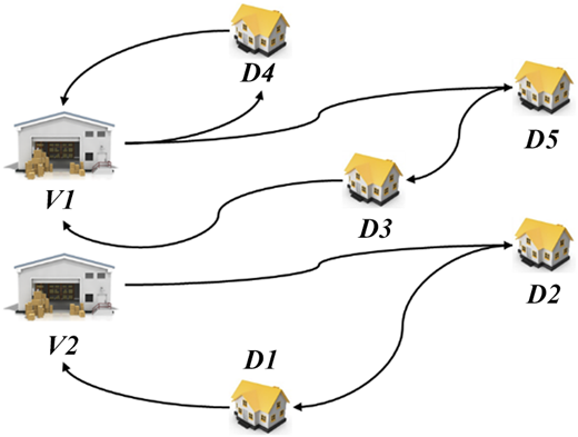
The graphical solution of the small size problem using GAMS software in the first period

Then the Pareto solutions of the model were obtained for ten different combinations of $γ_{n}$ (Table 5) that decision-maker can consider a range of different answers according to the condition and priorities of the objective functions.

Table 5

Pareto solutions of LP-metrics method

Assigned weights			Objective function solutions
$γ_{3}$	$γ_{2}$	$γ_{1}$	Total cost	Mean weighted response time	Waiting time
0.05	0.05	0.9	4000758.995	5.6	4.640
0.1	0.1	0.8	4048236.710	2.8	0.415
0.1	0.2	0.7	4060115.210	2.5	0.203
0.2	0.2	0.6	4060115.210	2.5	0.203
0.05	0.9	0.05	4060415.110	2.3	0.203
0.2	0.7	0.1	4062115.210	2.3	0.182
0.9	0.05	0.05	4078236.110	7.5	0.161
0.7	0.2	0.1	4060415.210	2.5	0.182
0.3	0.5	0.2	4060415.210	2.3	0.203
0.5	0.2	0.3	4060415.110	2.5	0.182

Assigned weights			Objective function solutions
$γ_{3}$	$γ_{2}$	$γ_{1}$	Total cost	Mean weighted response time	Waiting time
0.05	0.05	0.9	4000758.995	5.6	4.640
0.1	0.1	0.8	4048236.710	2.8	0.415
0.1	0.2	0.7	4060115.210	2.5	0.203
0.2	0.2	0.6	4060115.210	2.5	0.203
0.05	0.9	0.05	4060415.110	2.3	0.203
0.2	0.7	0.1	4062115.210	2.3	0.182
0.9	0.05	0.05	4078236.110	7.5	0.161
0.7	0.2	0.1	4060415.210	2.5	0.182
0.3	0.5	0.2	4060415.210	2.3	0.203
0.5	0.2	0.3	4060415.110	2.5	0.182

Furthermore, the results of solving the small-scale problem (for more information check Table A1) using the GOA algorithm are also given in Table 6 and the allocated routes in Figure 7. The values of the objective functions are 4156541.08, 2.3, and 0.231, respectively, with the allocation of 3 and 2 servers to the first and second warehouses. The results indicate a negligible difference in the outcomes of the GOA algorithm and the exact method.

Table 6

Optimal solution for small-scale example by the meta-heuristic algorithm

The average waiting time in the system		The average waiting time in the queue		The average number of vehicles in the system		The average number of vehicles in the queue		Probability of existence of 0 vehicles in the system
$w_{11}$	0.676	$w q_{11}$	0.0092	$L_{11}$	0.675	$L q_{11}$	0.0092	$π_{0}^{11}$	0.512
$w_{12}$	0.615	$w q_{12}$	0.0084	$L_{12}$	0.675	$L q_{12}$	0.0092	$π_{0}^{21}$	0.500
$w_{13}$	0.563	$w q_{13}$	0.0077	$L_{13}$	0.675	$L q_{13}$	0.0092	$π_{0}^{12}$	0.512
$w_{21}$	0.499	$w q_{21}$	0.0055	$L_{21}$	0.749	$L q_{21}$	0.0828	$π_{0}^{22}$	0.500
$w_{22}$	1.070	$w q_{22}$	0.1183	$L_{22}$	0.749	$L q_{22}$	0.0828	$π_{0}^{13}$	0.512
$w_{23}$	0.749	$w q_{23}$	0.0828	$L_{23}$	0.749	$L q_{23}$	0.0828	$π_{0}^{23}$	0.500

The average waiting time in the system		The average waiting time in the queue		The average number of vehicles in the system		The average number of vehicles in the queue		Probability of existence of 0 vehicles in the system
$w_{11}$	0.676	$w q_{11}$	0.0092	$L_{11}$	0.675	$L q_{11}$	0.0092	$π_{0}^{11}$	0.512
$w_{12}$	0.615	$w q_{12}$	0.0084	$L_{12}$	0.675	$L q_{12}$	0.0092	$π_{0}^{21}$	0.500
$w_{13}$	0.563	$w q_{13}$	0.0077	$L_{13}$	0.675	$L q_{13}$	0.0092	$π_{0}^{12}$	0.512
$w_{21}$	0.499	$w q_{21}$	0.0055	$L_{21}$	0.749	$L q_{21}$	0.0828	$π_{0}^{22}$	0.500
$w_{22}$	1.070	$w q_{22}$	0.1183	$L_{22}$	0.749	$L q_{22}$	0.0828	$π_{0}^{13}$	0.512
$w_{23}$	0.749	$w q_{23}$	0.0828	$L_{23}$	0.749	$L q_{23}$	0.0828	$π_{0}^{23}$	0.500

Probability of existence of n vehicles		Probability of existence of n vehicles		Probability of existence of n vehicles		Response time
$π_{1}^{11}$	0.341	$π_{3}^{21}$	0.037	$π_{6}^{11}$	3*10⁻⁴	$r_{121}$	4
$π_{1}^{12}$	0.341	$π_{3}^{22}$	0.037	$π_{6}^{12}$	3*10⁻⁴	$r_{122}$	1
$π_{1}^{13}$	0.341	$π_{3}^{23}$	0.037	$π_{6}^{13}$	3*10⁻⁴	$r_{123}$	1
$π_{1}^{21}$	0.333	$π_{4}^{11}$	0.005	$π_{6}^{21}$	0.001	$r_{221}$	2
$π_{1}^{22}$	0.333	$π_{4}^{12}$	0.005	$π_{6}^{22}$	0.001	$r_{222}$	2
$π_{1}^{23}$	0.333	$π_{4}^{13}$	0.005	$π_{6}^{23}$	0.001	$r_{223}$	2
$π_{2}^{11}$	0.113	$π_{4}^{21}$	0.012	$π_{7}^{11}$	0.0671*10⁻³	$r_{311}$	3
$π_{2}^{12}$	0.113	$π_{4}^{22}$	0.012	$π_{7}^{12}$	0.0617*10⁻³	$r_{312}$	4
$π_{2}^{13}$	0.113	$π_{4}^{23}$	0.012	$π_{7}^{13}$	0.0617*10⁻³	$r_{313}$	4
$π_{2}^{21}$	0.111	$π_{5}^{11}$	0.001	$π_{7}^{21}$	0.4573*10⁻³	$r_{411}$	2
$π_{2}^{22}$	0.111	$π_{5}^{12}$	0.001	$π_{7}^{22}$	0.4573*10⁻³	$r_{412}$	2
$π_{2}^{23}$	0.111	$π_{5}^{13}$	0.001	$π_{7}^{23}$	0.4573*10⁻³	$r_{413}$	2
$π_{3}^{11}$	0.025	$π_{5}^{21}$	0.004	$π_{8}^{21}$	0.1524*10⁻³	$r_{511}$	1
$π_{3}^{12}$	0.025	$π_{5}^{22}$	0.004	$π_{8}^{22}$	0.1524*10⁻³	$r_{512}$	1
$π_{3}^{13}$	0.025	$π_{5}^{23}$	0.004	$π_{8}^{23}$	0.1524*10⁻³	$r_{513}$	1

Probability of existence of n vehicles		Probability of existence of n vehicles		Probability of existence of n vehicles		Response time
$π_{1}^{11}$	0.341	$π_{3}^{21}$	0.037	$π_{6}^{11}$	3*10⁻⁴	$r_{121}$	4
$π_{1}^{12}$	0.341	$π_{3}^{22}$	0.037	$π_{6}^{12}$	3*10⁻⁴	$r_{122}$	1
$π_{1}^{13}$	0.341	$π_{3}^{23}$	0.037	$π_{6}^{13}$	3*10⁻⁴	$r_{123}$	1
$π_{1}^{21}$	0.333	$π_{4}^{11}$	0.005	$π_{6}^{21}$	0.001	$r_{221}$	2
$π_{1}^{22}$	0.333	$π_{4}^{12}$	0.005	$π_{6}^{22}$	0.001	$r_{222}$	2
$π_{1}^{23}$	0.333	$π_{4}^{13}$	0.005	$π_{6}^{23}$	0.001	$r_{223}$	2
$π_{2}^{11}$	0.113	$π_{4}^{21}$	0.012	$π_{7}^{11}$	0.0671*10⁻³	$r_{311}$	3
$π_{2}^{12}$	0.113	$π_{4}^{22}$	0.012	$π_{7}^{12}$	0.0617*10⁻³	$r_{312}$	4
$π_{2}^{13}$	0.113	$π_{4}^{23}$	0.012	$π_{7}^{13}$	0.0617*10⁻³	$r_{313}$	4
$π_{2}^{21}$	0.111	$π_{5}^{11}$	0.001	$π_{7}^{21}$	0.4573*10⁻³	$r_{411}$	2
$π_{2}^{22}$	0.111	$π_{5}^{12}$	0.001	$π_{7}^{22}$	0.4573*10⁻³	$r_{412}$	2
$π_{2}^{23}$	0.111	$π_{5}^{13}$	0.001	$π_{7}^{23}$	0.4573*10⁻³	$r_{413}$	2
$π_{3}^{11}$	0.025	$π_{5}^{21}$	0.004	$π_{8}^{21}$	0.1524*10⁻³	$r_{511}$	1
$π_{3}^{12}$	0.025	$π_{5}^{22}$	0.004	$π_{8}^{22}$	0.1524*10⁻³	$r_{512}$	1
$π_{3}^{13}$	0.025	$π_{5}^{23}$	0.004	$π_{8}^{23}$	0.1524*10⁻³	$r_{513}$	1

Figure 7

View large Download slide

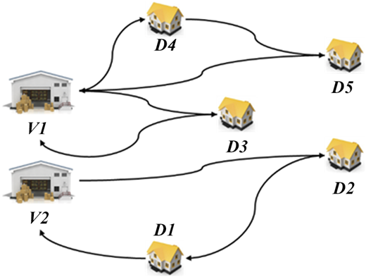
The graphical solution of the small-scale problem using GOA in the first period

6.1.2 Comparative study

Table 7 tabulates a comparative study of the results of solving three random models with GAMS and GOA. These data sets are obtained by increasing the size of a small problem, and due to the increasing trend of the computational time of solving problems by the exact method, it is not logical to use GAMs for large-size problems. Hence it is more efficient to use a meta-heuristic algorithm. To determine the efficiency of the proposed algorithm, a gap between GAMS and GOA algorithm is presented in equation (38).

Gap (%) = \frac{100 * (Z_{GAMS} - Z_{GOA})}{Z_{GOA}}

(38)

Table 7

Comparison the results of GOA with GAMS for small-scale problems

Data set	Z	Value of objective functions		CPU engagement time		Gap%
Data set	Z	GAMS	GOA	GAMS	GOA	Gap%
1	Z1	1674447.94	1733200	00:00:01	00:00:04	3.38
	Z2	2.6	2.6			0.00
	Z3	0.171	0.171			0.00
2	Z1	4060414.910	4156541.08	00:00:13	00:00:04	2.31
	Z2	2.3	2.3			0.00
	Z3	0.203	0.211			3.79
3	Z1	6450754.152	6822214.12	00:16:42	00:00:04	5.44
	Z2	2.3	2.3			0.00
	Z3	0.354	0.354			0.00

Data set	Z	Value of objective functions		CPU engagement time		Gap%
Data set	Z	GAMS	GOA	GAMS	GOA	Gap%
1	Z1	1674447.94	1733200	00:00:01	00:00:04	3.38
	Z2	2.6	2.6			0.00
	Z3	0.171	0.171			0.00
2	Z1	4060414.910	4156541.08	00:00:13	00:00:04	2.31
	Z2	2.3	2.3			0.00
	Z3	0.203	0.211			3.79
3	Z1	6450754.152	6822214.12	00:16:42	00:00:04	5.44
	Z2	2.3	2.3			0.00
	Z3	0.354	0.354			0.00

In which, $Z_{GAMS}$ and $Z_{GOA}$ are the objective function values of optimal solutions over the GAMS and GOA, respectively. According to the obtained gaps in Table 7, there is no significant difference between GAMS and GOA results, and the proposed algorithm is qualified. Hence, it can be concluded that the GOA can be used for large-scale problems.

6.1.3 Large-scale problem

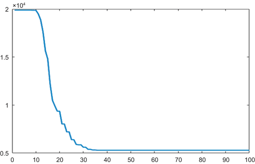
The results of solving the large-scale instance (for more information check Table A2) using the GOA algorithm are also shown in Table 8, and the problem-solving convergence diagram for the large example is demonstrated in Figure 8. A preview of the routing results has provided in Figure A1.

Table 8

Optimal solution for large-scale problem using GOA

Objective functions	Values
Total cost	1.2628 × 10¹¹	1.2866 × 10¹¹	1.2723 × 10¹¹	1.2674 × 10¹¹	1.2744 × 10¹¹
Average waiting time	861.4256	856.5014	848.3892	822.1576	821.3063
Total weighted response time	50.9548	34.2033	41.3147	60.1843	36.8671

Objective functions	Values
Total cost	1.2628 × 10¹¹	1.2866 × 10¹¹	1.2723 × 10¹¹	1.2674 × 10¹¹	1.2744 × 10¹¹
Average waiting time	861.4256	856.5014	848.3892	822.1576	821.3063
Total weighted response time	50.9548	34.2033	41.3147	60.1843	36.8671

Figure 8

View large Download slide

Convergence of GOA to the optimal solution for large size example

Figure A1

View large Download slide

Large-scale problem routing preview

6.2 Case study

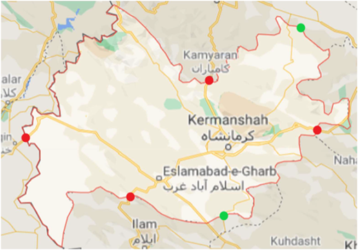
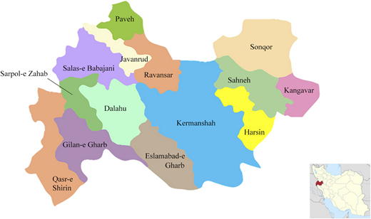
Kermanshah is located on four major faults (Mountain front, High Zagros, Sahneh and Morvarid), so lots of earthquakes threaten this province. Therefore, in this section, we implemented our model to the Kermanshah earthquake in 2017 and solved it using GOA. Kermanshah province is bound by three provinces of Iran and by Iraq on the west. There are several entrances to this province which 6 entrances are selected for locating border warehouses and are marked by red and green bullets in Figure 9. Two types of items are considered as relief goods in this model: Food and water which are distributed among demand points by two types of transportation modes: pickup trucks and light transportation helicopters. Also, arrival vehicles are including heavy transportation helicopters and trucks. In this case, red bullets indicate the designated warehouses for trucks and in the same way, green dots relate to helicopters (Figure 9). As is illustrated in Figure 10, this province is divided into 14 counties which the center of each county is designated for delivery of relief goods. The distances and traveling time between warehouses and demand points are calculated by Google map's measure tool. It should be noted that the demand of each county is assumed to be equal to the population of that county and the population of each county is obtained through statistics prepared by the Statistical Center of Iran (National Statistical Center of Iran, 2019). Furthermore, the weights of demand points are calculated due to the population rate of the counties in which Sarpol Zahab was the most critical based on that (more information is proposed in Appendix, Table A6). Relating data to the case study is prepared in Appendix section (Tables A3–A5). Pareto solutions of implementing the proposed model on the case study are provided in Table 9 and optimal values for the number of servers as well as assigned demand points to the warehouses for the first run of the meta-heuristic algorithm are demonstrated in Table 10. Due to the large number of servers in each warehouse, the waiting time of vehicles in the queues is not so long, in this case, decision-makers can define upper bounds for the number of servers according to conditions and limitations.

Figure 9

View large Download slide

Location of border warehouses

Figure 10

View large Download slide

Counties of Kermanshah province

Table A6

Population and weight of counties

County	Population	Weight
Kermanshah	1083,833	0.04
Kangavar	76,216	0.04
Sonqor	81,661	0.04
Sahneh	70,757	0.04
Harsin	78,350	0.04
Javanrud	75,169	0.1
Eslamabad-e-gharrb	140,876	0.04
Gilangharb	57,007	0.1
Sarpol Zahab	85,342	0.2
Qasre shirin	23,929	0.1
Paveh	60,431	0.04
Ravansar	47,657	0.04
Dalahu	35,987	0.08
Salas Babajani	35,219	0.1

County	Population	Weight
Kermanshah	1083,833	0.04
Kangavar	76,216	0.04
Sonqor	81,661	0.04
Sahneh	70,757	0.04
Harsin	78,350	0.04
Javanrud	75,169	0.1
Eslamabad-e-gharrb	140,876	0.04
Gilangharb	57,007	0.1
Sarpol Zahab	85,342	0.2
Qasre shirin	23,929	0.1
Paveh	60,431	0.04
Ravansar	47,657	0.04
Dalahu	35,987	0.08
Salas Babajani	35,219	0.1

Table A3

Distance between warehouses and counties (kms)

	Entrance 5	Entrance 6	Kermanshah	Kangavar	Sonqor	Sahneh	Harsin	Javanrud	Eslamabad-e-gharrb	Gilangharb	Sarpol Zahab	Qasre shirin	Paveh	Ravansar	Dalahu	Salas Babajani
Entrance 1	–	–	63.21	141	95.8	110	111	62.5	115	196	198	225	93.8	39.8	93.5	113
Entrance 2	–	–	99.3	197	193	166	157	131	33.1	48.6	78.8	104	177	122	66.4	150
Entrance 3	–	–	74	21.8	60.9	10.1	65.3	174	142	222	301	252	205	141	151	211
Entrance 4	–	–	197	295	291	264	255	160	128	76.9	51.4	20.5	205	194	149	113
Kermanshah	199.3	69.0	–	95	93.6	63.9	56.8	92.8	67	148	150	177	124	69.2	73.4	133
Kangavar	130.3	161.0	95	–	80.3	31.4	93.3	180	165	245	247	275	211	157	174	230
Sonqor	103.5	161.0	93.6	80.3	–	53.2	90.4	150	162	242	243	272	181	128	170	202
Sahneh	161.0	130.3	63.9	31.4	53.2	–	62.7	150	134	215	217	244	181	126	144	199
Harsin	195.5	122.7	56.8	93.3	90.4	62.7	–	141	125	206	208	235	172	117	135	190
Javanrud	210.8	153.3	92.8	180	150	150	141	–	98.6	179	121	141	44.6	24	62.4	54.5
Eslamabad-e-gharrb	264.5	61.3	67	165	162	134	125	98.6	–	81.4	81	108	157	101	63.3	119
Gilangharb	348.8	141.8	148	245	242	215	206	179	81.4	–	53.5	56.8	226	171	143	124
Sarpol Zahab	348.8	145.7	150	247	243	217	208	121	81	53.5	–	31.6	204	148	103	73.4
Qasre shirin	375.7	172.5	177	275	272	244	235	141	108	56.8	31.6	–	185	177	133	92.7
Paveh	241.5	195.5	124	211	181	181	172	44.6	157	226	204	185	–	55.5	109	98.9
Ravansar	187.8	145.7	69.2	157	128	126	117	24	101	171	148	177	55.5	–	53.9	73.6
Dalahu	241.5	126.5	73.4	174	170	144	135	62.4	63.3	143	103	133	109	53.9	–	67.6
Salas Babajani	260.7	191.7	133	230	202	199	190	54.5	119	124	73.4	92.7	98.9	73.6	67.6	–

	Entrance 5	Entrance 6	Kermanshah	Kangavar	Sonqor	Sahneh	Harsin	Javanrud	Eslamabad-e-gharrb	Gilangharb	Sarpol Zahab	Qasre shirin	Paveh	Ravansar	Dalahu	Salas Babajani
Entrance 1	–	–	63.21	141	95.8	110	111	62.5	115	196	198	225	93.8	39.8	93.5	113
Entrance 2	–	–	99.3	197	193	166	157	131	33.1	48.6	78.8	104	177	122	66.4	150
Entrance 3	–	–	74	21.8	60.9	10.1	65.3	174	142	222	301	252	205	141	151	211
Entrance 4	–	–	197	295	291	264	255	160	128	76.9	51.4	20.5	205	194	149	113
Kermanshah	199.3	69.0	–	95	93.6	63.9	56.8	92.8	67	148	150	177	124	69.2	73.4	133
Kangavar	130.3	161.0	95	–	80.3	31.4	93.3	180	165	245	247	275	211	157	174	230
Sonqor	103.5	161.0	93.6	80.3	–	53.2	90.4	150	162	242	243	272	181	128	170	202
Sahneh	161.0	130.3	63.9	31.4	53.2	–	62.7	150	134	215	217	244	181	126	144	199
Harsin	195.5	122.7	56.8	93.3	90.4	62.7	–	141	125	206	208	235	172	117	135	190
Javanrud	210.8	153.3	92.8	180	150	150	141	–	98.6	179	121	141	44.6	24	62.4	54.5
Eslamabad-e-gharrb	264.5	61.3	67	165	162	134	125	98.6	–	81.4	81	108	157	101	63.3	119
Gilangharb	348.8	141.8	148	245	242	215	206	179	81.4	–	53.5	56.8	226	171	143	124
Sarpol Zahab	348.8	145.7	150	247	243	217	208	121	81	53.5	–	31.6	204	148	103	73.4
Qasre shirin	375.7	172.5	177	275	272	244	235	141	108	56.8	31.6	–	185	177	133	92.7
Paveh	241.5	195.5	124	211	181	181	172	44.6	157	226	204	185	–	55.5	109	98.9
Ravansar	187.8	145.7	69.2	157	128	126	117	24	101	171	148	177	55.5	–	53.9	73.6
Dalahu	241.5	126.5	73.4	174	170	144	135	62.4	63.3	143	103	133	109	53.9	–	67.6
Salas Babajani	260.7	191.7	133	230	202	199	190	54.5	119	124	73.4	92.7	98.9	73.6	67.6	–

Table A4

Required time to transfer between warehouses and counties by truck (hours)

	Kermanshah	Kangavar	Sonqor	Sahneh	Harsin	Javanrud	Eslamabad-e-gharrb	Gilangharb	Sarpol Zahab	Qasre shirin	Paveh	Ravansar	Dalahu	Salas Babajani
Entrance 1	1:06	2:09	1:31	1:43	1:42	1:17	1:36	2:47	2:34	2:56	1:52	0:51	1:43	2:41
Entrance 2	1:25	2:36	2:36	2:08	2:05	1:53	0:32	0:48	1:12	1:30	2:47	1:43	0:54	2:36
Entrance 3	0:22	1:04	0:11	0:56	2:39	1:54	2:58	4:32	3.04	3:14	1:52	2:10	3:10	0:22
Entrance 4	2:35	3:50	3:50	3:22	3:18	2:50	1:40	1:08	0:48	0:20	3:48	2:56	2:15	1:58
Kermanshah	–	1:21	1:23	0:56	0:54	1:25	1:00	2:11	1:57	2:18	1:59	0:59	1:14	2:16
Kangavar	1:21	–	1:08	0:31	1:18	2:33	2:10	3:22	3:11	3:32	3:07	2:07	2:29	3:29
Sonqor	1:23	1:08	–	0:52	1:20	2:22	2:12	3:19	3:05	3:26	2:57	1:57	2:30	3:17
Sahneh	0:56	0:31	0:52	–	0:53	2:08	1:45	2:58	2:46	3:07	2:42	1:42	2:04	3:04
Harsin	0:54	1:18	1:20	0:53	–	2:05	1:41	2:54	2:42	3:03	2:39	1:39	2:00	2:59
Javanrud	1:25	2:33	2:22	2:08	2:05	–	1:28	2:40	2:21	2:33	0:59	0:28	1:02	1:05
Eslamabad-e-gharrb	1:00	2:10	2:12	1:45	1:41	1:28	–	1:18	1:02	1:23	2:30	1:29	1:01	2:18
Gilangharb	2:11	3:22	3:19	2:58	2:54	2:40	1:18	–	0:54	0:50	3:34	2:31	2:12	2:14
Sarpol Zahab	1:57	3:11	3:05	2:46	2:42	2:21	1:02	0:54	–	0:30	3:19	2:19	1:39	1:32
Qasre shirin	2:18	3:32	3:26	3:07	3:03	2:33	1:23	0:50	0:30	–	3:31	2:40	2:00	1:44
Paveh	1:59	3:07	2:57	2:42	2:39	0:59	2:30	3:34	3:19	3:31	–	1:02	1:54	2:01
Ravansar	0:59	2:07	1:57	1:42	1:39	0:28	1:29	2:31	2:19	2:40	1:02	–	0:53	1:21
Dalahu	1:14	2:29	2:30	2:04	2:00	1:02	1:01	2:12	1:39	2:00	1:54	0:53	–	1:37
Salas Babajani	2:16	3:29	3:17	3:04	2:59	1:05	2:18	2:14	1:32	1:44	2:01	1:21	1:37	–

	Kermanshah	Kangavar	Sonqor	Sahneh	Harsin	Javanrud	Eslamabad-e-gharrb	Gilangharb	Sarpol Zahab	Qasre shirin	Paveh	Ravansar	Dalahu	Salas Babajani
Entrance 1	1:06	2:09	1:31	1:43	1:42	1:17	1:36	2:47	2:34	2:56	1:52	0:51	1:43	2:41
Entrance 2	1:25	2:36	2:36	2:08	2:05	1:53	0:32	0:48	1:12	1:30	2:47	1:43	0:54	2:36
Entrance 3	0:22	1:04	0:11	0:56	2:39	1:54	2:58	4:32	3.04	3:14	1:52	2:10	3:10	0:22
Entrance 4	2:35	3:50	3:50	3:22	3:18	2:50	1:40	1:08	0:48	0:20	3:48	2:56	2:15	1:58
Kermanshah	–	1:21	1:23	0:56	0:54	1:25	1:00	2:11	1:57	2:18	1:59	0:59	1:14	2:16
Kangavar	1:21	–	1:08	0:31	1:18	2:33	2:10	3:22	3:11	3:32	3:07	2:07	2:29	3:29
Sonqor	1:23	1:08	–	0:52	1:20	2:22	2:12	3:19	3:05	3:26	2:57	1:57	2:30	3:17
Sahneh	0:56	0:31	0:52	–	0:53	2:08	1:45	2:58	2:46	3:07	2:42	1:42	2:04	3:04
Harsin	0:54	1:18	1:20	0:53	–	2:05	1:41	2:54	2:42	3:03	2:39	1:39	2:00	2:59
Javanrud	1:25	2:33	2:22	2:08	2:05	–	1:28	2:40	2:21	2:33	0:59	0:28	1:02	1:05
Eslamabad-e-gharrb	1:00	2:10	2:12	1:45	1:41	1:28	–	1:18	1:02	1:23	2:30	1:29	1:01	2:18
Gilangharb	2:11	3:22	3:19	2:58	2:54	2:40	1:18	–	0:54	0:50	3:34	2:31	2:12	2:14
Sarpol Zahab	1:57	3:11	3:05	2:46	2:42	2:21	1:02	0:54	–	0:30	3:19	2:19	1:39	1:32
Qasre shirin	2:18	3:32	3:26	3:07	3:03	2:33	1:23	0:50	0:30	–	3:31	2:40	2:00	1:44
Paveh	1:59	3:07	2:57	2:42	2:39	0:59	2:30	3:34	3:19	3:31	–	1:02	1:54	2:01
Ravansar	0:59	2:07	1:57	1:42	1:39	0:28	1:29	2:31	2:19	2:40	1:02	–	0:53	1:21
Dalahu	1:14	2:29	2:30	2:04	2:00	1:02	1:01	2:12	1:39	2:00	1:54	0:53	–	1:37
Salas Babajani	2:16	3:29	3:17	3:04	2:59	1:05	2:18	2:14	1:32	1:44	2:01	1:21	1:37	–

Table A5

Required time to transfer between warehouses and counties by helicopter (hours)

	Entrance 5	Entrance 6	Kermanshah	Kangavar	Sonqor	Sahneh	Harsin	Javanrud	Eslamabad-e-gharrb	Gilangharb	Sarpol Zahab	Qasre shirin	Paveh	Ravansar	Dalahu	Salas Babajani
Kermanshah	0:52	0:18	–	0:24	0:24	0:16	0:14	0:24	0:17	0:38	0:39	0:46	0:32	0:18	0:19	0:34
Kangavar	0:34	0:42	0:24	–	0:20	0:08	0:24	0:46	0:43	1:03	1:04	1:11	0:55	0:40	0:45	1:00
Sonqor	0:27	0:42	0:24	0:20	–	0:13	0:23	0:39	0:42	1:03	1:03	1:10	0:47	0:33	0:44	0:52
Sahneh	0:42	0:34	0:16	0:08	0:13	–	0:16	0:39	0:34	0:56	0:56	1:03	0:47	0:32	0:37	0:51
Harsin	0:51	0:32	0:14	0:24	0:23	0:16	–	0:36	0:32	0:53	0:54	1:01	0:44	0:30	0:35	0:49
Javanrud	0:55	0:40	0:24	0:46	0:39	0:39	0:36	–	0:25	0:46	0:31	0:36	0:11	0:06	0:16	0:14
Eslamabad-e-gharrb	1:09	0:16	0:17	0:43	0:42	0:34	0:32	0:25	–	0:21	0:21	0:28	0:40	0:26	0:16	0:31
Gilangharb	1:31	0:37	0:38	1:03	1:03	0:56	0:53	0:46	0:21	–	0:13	0:14	0:58	0:44	0:37	0:32
Sarpol Zahab	1:31	0:38	0:39	1:04	1:03	0:56	0:54	0:31	0:21	0:13	–	0:08	0:53	0:38	0:26	0:19
Qasre shirin	1:38	0:45	0:46	1:11	1:10	1:03	1:01	0:36	0:28	0:14	0:08	–	0:48	0:46	0:34	0:24
Paveh	1:03	0:51	0:32	0:55	0:47	0:47	0:44	0:11	0:40	0:58	0:53	0:48	–	0:14	0:28	0:25
Ravansar	0:49	0:38	0:18	0:40	0:33	0:32	0:30	0:06	0:26	0:44	0:38	0:46	0:14	–	0:14	0:19
Dalahu	1:03	0:33	0:19	0:45	0:44	0:37	0:35	0:16	0:16	0:37	0:26	0:34	0:28	0:14	–	0:17
Salas Babajani	1:08	0:50	0:34	1:00	0:52	0:51	0:49	0:14	0:31	0:32	0:19	0:24	0:25	0:19	0:17	–

	Entrance 5	Entrance 6	Kermanshah	Kangavar	Sonqor	Sahneh	Harsin	Javanrud	Eslamabad-e-gharrb	Gilangharb	Sarpol Zahab	Qasre shirin	Paveh	Ravansar	Dalahu	Salas Babajani
Kermanshah	0:52	0:18	–	0:24	0:24	0:16	0:14	0:24	0:17	0:38	0:39	0:46	0:32	0:18	0:19	0:34
Kangavar	0:34	0:42	0:24	–	0:20	0:08	0:24	0:46	0:43	1:03	1:04	1:11	0:55	0:40	0:45	1:00
Sonqor	0:27	0:42	0:24	0:20	–	0:13	0:23	0:39	0:42	1:03	1:03	1:10	0:47	0:33	0:44	0:52
Sahneh	0:42	0:34	0:16	0:08	0:13	–	0:16	0:39	0:34	0:56	0:56	1:03	0:47	0:32	0:37	0:51
Harsin	0:51	0:32	0:14	0:24	0:23	0:16	–	0:36	0:32	0:53	0:54	1:01	0:44	0:30	0:35	0:49
Javanrud	0:55	0:40	0:24	0:46	0:39	0:39	0:36	–	0:25	0:46	0:31	0:36	0:11	0:06	0:16	0:14
Eslamabad-e-gharrb	1:09	0:16	0:17	0:43	0:42	0:34	0:32	0:25	–	0:21	0:21	0:28	0:40	0:26	0:16	0:31
Gilangharb	1:31	0:37	0:38	1:03	1:03	0:56	0:53	0:46	0:21	–	0:13	0:14	0:58	0:44	0:37	0:32
Sarpol Zahab	1:31	0:38	0:39	1:04	1:03	0:56	0:54	0:31	0:21	0:13	–	0:08	0:53	0:38	0:26	0:19
Qasre shirin	1:38	0:45	0:46	1:11	1:10	1:03	1:01	0:36	0:28	0:14	0:08	–	0:48	0:46	0:34	0:24
Paveh	1:03	0:51	0:32	0:55	0:47	0:47	0:44	0:11	0:40	0:58	0:53	0:48	–	0:14	0:28	0:25
Ravansar	0:49	0:38	0:18	0:40	0:33	0:32	0:30	0:06	0:26	0:44	0:38	0:46	0:14	–	0:14	0:19
Dalahu	1:03	0:33	0:19	0:45	0:44	0:37	0:35	0:16	0:16	0:37	0:26	0:34	0:28	0:14	–	0:17
Salas Babajani	1:08	0:50	0:34	1:00	0:52	0:51	0:49	0:14	0:31	0:32	0:19	0:24	0:25	0:19	0:17	–

Table 9

Pareto solutions of case study

	Total cost (Rials)	Average weighted response time (hours)	Total waiting time for vehicles (hours)
1	1.28 × 10¹¹	1.57	6.6
2	1.30 × 10¹¹	1.39	7.1
3	1.34 × 10¹¹	1.24	5.9
4	1.32 × 10¹¹	1.46	6.7
5	1.29 × 10¹¹	1.48	6.7

	Total cost (Rials)	Average weighted response time (hours)	Total waiting time for vehicles (hours)
1	1.28 × 10¹¹	1.57	6.6
2	1.30 × 10¹¹	1.39	7.1
3	1.34 × 10¹¹	1.24	5.9
4	1.32 × 10¹¹	1.46	6.7
5	1.29 × 10¹¹	1.48	6.7

Table 10

Optimal decision variables for the first run

Number of optimal servers	S1	S2	S3	S4	S5	S6
Number of optimal servers	12	2	19	4	14	20
Assigned counties to servers (first period)	(11,4,1)	(9,3,7)	(10,12,14)	(8,5,13)	(−)	(6,2)
Assigned counties to servers (second period)	(12)	(11,10)	(8,6,2,7,9)	(13,14,1)	(5,3,4)	(−)
Assigned counties to servers (third period)	(−)	(6,13,9,12)	(11,10,3,8,2)	(4,14)	(5,7)	(1)

Number of optimal servers	S1	S2	S3	S4	S5	S6
Number of optimal servers	12	2	19	4	14	20
Assigned counties to servers (first period)	(11,4,1)	(9,3,7)	(10,12,14)	(8,5,13)	(−)	(6,2)
Assigned counties to servers (second period)	(12)	(11,10)	(8,6,2,7,9)	(13,14,1)	(5,3,4)	(−)
Assigned counties to servers (third period)	(−)	(6,13,9,12)	(11,10,3,8,2)	(4,14)	(5,7)	(1)

6.3 Sensitivity analysis

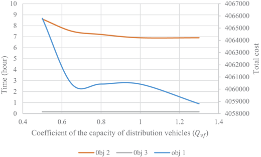
To find the effective parameters and show their effect on the optimal answer and objective functions as well as better understanding of the model behavior, sensitivity analysis has been performed. The results of the sensitivity analysis are given in Figures 11–15. Figure 11 demonstrates the effects of the capacity of distribution vehicles on the objective functions. This diagram illustrates that the third objective function is not sensitive to the capacity of the transport vehicles and the first and second objective functions have a decreasing trend with increasing the capacity of the vehicles. Expanding the capacity reduces the number of vehicles needed for distribution, thus lessen the routing costs. The distance between the border warehouses and the damaged areas is very large due to the importance of the security of the warehouses. Therefore, if each vehicle can deliver more items, the time spent transporting items from warehouses to disaster areas will be reduced, which will improve the function of the second objective of the problem. As a result, decision-makers can use vehicles with optimal capacity according to the conditions.

Figure 11

View large Download slide

Coefficient of the capacity of distribution vehicles vs objective functions

Figure 12

View large Download slide

Arrival rate of vehicles vs first and third objective functions

Figure 13

View large Download slide

Arrival rate of vehicles vs number of assigned servers

Figure 14

View large Download slide

The capacity of waiting space vs waiting time of vehicles in the queue and number of servers

Figure 15

View large Download slide

Range of $λ_{v t}$ vs total inventory

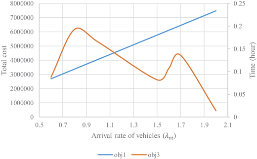
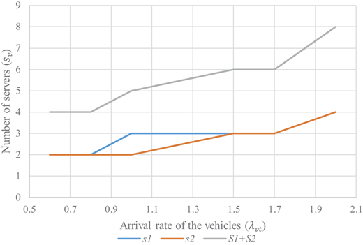
The results of the changes in $λ_{v t}$ ⁠, which indicate the entry rate of vehicles into warehouses, on the system outlays and the average waiting time of vehicles in the queue is displayed in Figure 12. With the enhancing rate of arrival of vehicles, the surplus inventory stored in warehouses also increased. Evidently, by adding the inventory stored in the warehouses, more costs will be imposed on the system to hold these items. Besides, the inventory holding cost per unit of time is a significant consideration to avoid storing essential items in warehouses during a disaster and prevent shortages in other locations by leveling resources. Figure 12 represents that with increasing $λ_{v t}$ ⁠, the graph of the third objective function has an upward trend in some periods, and at certain intervals, the trend is declining. According to Figure 13, it is inferred that with the growth in the arrival rate of vehicles to warehouses, in the case that the number of warehouse servers is assumed to be constant, the third objective function has a rising trend and if the number of servers increases, the third objective function will improve.

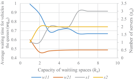
As expressed in Table 11 and Figure 14, changes in the capacity of the waiting space of warehouses have significant consequences on the average waiting time for vehicles in addition to system costs. According to Table 11, capacity enhancement leads to enter more vehicles which adding more servers to the warehouses reduces the congestion. But due to the assumed fixed value for entry rate in this example, increasing the capacity of waiting spaces will not always affect the entry rate, and it remains constant after a point such as the 5th row in Table 11. Hence, the number of servers and, consequently, the waiting time of vehicles will eventually remain constant as K increases. On the other hand, increasing the number of servers increases the number of goods stored in the warehouses and leads to ascending inventory cost behavior. But by stabilizing the number of servers, this ascending trend is not sharp. An increment in the capacity of the warehouses directly affects the optimal number of servers, and consequently, the average waiting time of the vehicles in the system also changes, according to Figure 14. This diagram represents the changes in the average waiting time of trucks in the queues in the first period.

Table 11

The capacity of waiting spaces vs total cost

mode	K1, K2	S1	S2	${\bar{λ}}_{11}$	${\bar{λ}}_{12}$	${\bar{λ}}_{13}$	${\bar{λ}}_{21}$	${\bar{λ}}_{22}$	${\bar{λ}}_{23}$	Total cost
1	1,2	1	1	0.349	0.383	0.418	0.730	0.353	0.495	2811413.7
2	2,3	1	2	0.359	0.391	0.424	0.770	0.363	0.516	3593069.801
3	3,4	2	2	0.503	0.553	0.602	0.763	0.362	0.512	3962061.853
4	4,5	2	2	0.508	0.558	0.608	0.761	0.361	0.511	4028292.427
5	5,6	2	2	0.509	0.559	0.610	0.761	0.362	0.511	4050061.998
6	6,7	3	2	0.514	0.566	0.617	0.761	0.362	0.511	4059284.406
7	7,8	3	2	0.514	0.566	0.617	0.761	0.362	0.511	4060415.11
8	11,12	3	2	0.514	0.566	0.617	0.761	0.362	0.511	4060890.501

mode	K1, K2	S1	S2	${\bar{λ}}_{11}$	${\bar{λ}}_{12}$	${\bar{λ}}_{13}$	${\bar{λ}}_{21}$	${\bar{λ}}_{22}$	${\bar{λ}}_{23}$	Total cost
1	1,2	1	1	0.349	0.383	0.418	0.730	0.353	0.495	2811413.7
2	2,3	1	2	0.359	0.391	0.424	0.770	0.363	0.516	3593069.801
3	3,4	2	2	0.503	0.553	0.602	0.763	0.362	0.512	3962061.853
4	4,5	2	2	0.508	0.558	0.608	0.761	0.361	0.511	4028292.427
5	5,6	2	2	0.509	0.559	0.610	0.761	0.362	0.511	4050061.998
6	6,7	3	2	0.514	0.566	0.617	0.761	0.362	0.511	4059284.406
7	7,8	3	2	0.514	0.566	0.617	0.761	0.362	0.511	4060415.11
8	11,12	3	2	0.514	0.566	0.617	0.761	0.362	0.511	4060890.501

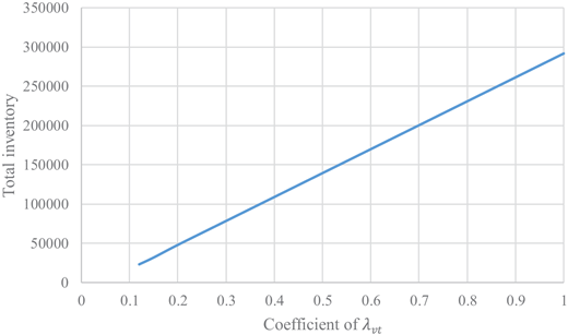
Figure 15 shows feasible ranges of $λ_{v t}$ and its effect on total inventory. To make the model feasible, $λ_{v t}$ must be within the specified range, for values less than the interval rate, the problem will face a shortage which is not allowed. Besides, large quantities of entry rate increase the inventory stored in the warehouses, although this volume of inventory improves responsiveness to injured people, but increases inventory holding.

6.4 Discussion

The model presented in this study allows decision-makers to consider all dimensions of the issue in terms of practical and managerial aspects and make decisions based on them at the time of the disaster. Numerous articles such as Suzuki (2019) and Rezaei-Malek et al. (2016) have been conducted in the field of humanitarian logistics, but these articles have not taken into account the importance and impact of congestion at the entry points of disaster areas. In this study, such as Rezaei-Malek et al. (2016), in addition to reducing the delivery time of essential items to the damaged areas, system outlays are also considered. The unmanaged congestion in border areas results in the increment in the unemployment time of vehicles in the queues, as well as the disorder in these areas, and consequently disrupts the passage of other relief vehicles. Using the queuing system in the proposed model helps to manage this density better and reduce it.

From a managerial point of view, according to the results obtained from Section 6.3, disaster managers and decision-makers should use vehicles with more capacity if it is possible to reduce congestion and operational costs. Also, they can prevent the congestion of vehicles in border warehouses by increasing the number of servers while the financial constraints are satisfied. On the other hand, increasing the entry rate by increasing space capacity and servers increases the inventory cost. Therefore, decision-makers can determine the optimal values by solving the proposed multi-objective model by their preferred weights. Finally, however, increasing the entry rate increases the inventory and response level to the affected people but causes inventory accumulation, which increases inventory holding cost. Also, it is better to use these extra inventories in another affected area, so decision-makers can direct the rest of the vehicles to other areas based on demand and by considering the appropriate level of safety stock.

7. Conclusion and future research

In this study, a mathematical model for multi-objective multi-commodity and multi-period inventory routing problems in post-disaster conditions is presented by considering the density of vehicles carrying relief items at the entrance of the border warehouses. For the first time in the logistics literature, the queuing system is included in the modeling framework in the areas affected by a disaster. Due to the limitation in the unloading rate of items in the warehouses, the entry flow to the warehouses must wait for the unloading in the queue. In this study, the capacity for the number of vehicles that can wait is confined. Therefore, the M/M/C/K queuing system was developed to analyze the waiting time at the warehouse entrance and the length of these queues. Efforts to reduce congestion at entry points will not only facilitate for other relief vehicles to pass through but will also leverage transportation resources. As a result, in addition to mitigating the cost and time of distribution of items between demand points, this model also seeks to reduce the average waiting time for vehicles in warehouses. Also, each warehouse is assigned a mode of transport (helicopters, trucks, etc.).

Furthermore, to solve larger problems, the GOA metaheuristic algorithm is used in this research, and comparing its results with the outcomes of GAMS software on small instances indicates the efficiency of this algorithm. Finally, sensitivity analyses were performed on the effective parameters of the model.

According to the results, increasing the capacity of distribution vehicles alleviates system costs and average weight delivery time. Also, the rate at which vehicles enter warehouses affects system costs, the optimal number of servers and the number of queues.

For future studies, it is recommended to enable split delivery. Decisions about the location of warehouses can also be added to the problem, as well as including capacity constraints for depots. By removing the limitation of shortages, the concept of social fairness can be added to the model. Another suggestion for future studies, which may be interesting, is to investigate the rejected trucks in the proposed model (for more information, refer to equation (1)). Also, we highly recommend that future researchers use multi-attribute decision-making (MADM) methods to obtain the weight of each demand point. Also, the loading servers may fail at any point in time. Hence, a server breakdown may stop the service of vehicles completely or lead to the service continuing at a slower rate (Aghsami and Jolai, 2020). Therefore, considering the loading serves breakdowns can be an interesting problem for future research.

The authors would like to thank the editor-in-chief and the anonymous reviewers for their valuable comments and helpful suggestions on a previous draft of this paper to improve its quality. This work was supported by the Iranian National Science Foundation (91049559).

References

Abazari

,

S.R.

,

Aghsami

,

A.

and

Rabbani

,

M.

(

2020

), “

Prepositioning and distributing relief items in humanitarian logistics with uncertain parameters

”,

Socio-Economic Planning Sciences

, Vol.

74

, pp.

1

-

17

, 100933, doi:

https://doi.org/10.1016/j.seps.2020.100933

.

Google Scholar

Crossref

Abualigah

,

L.

and

Diabat

,

A.

(

2020

), “

A comprehensive survey of the Grasshopper optimization algorithm: results, variants, and applications

”,

Neural Computing and Applications

, Vol.

32

, pp.

15533

-

15556

, doi:

https://doi.org/10.1007/s00521-020-04789-8

.

Google Scholar

Crossref

Aghsami

,

A.

and

Jolai

,

F.

(

2020

), “

Equilibrium threshold strategies and social benefits in the fully observable Markovian queues with partial breakdowns and interruptible setup/closedown policy

”,

Quality Technology and Quantitative Management

, Vol.

17

No.

6

, pp.

685

-

722

, doi:

https://doi.org/10.1080/16843703.2020.1736365

.

Google Scholar

Crossref

Ahmadi

,

A.

and

Bazargan-Hejazi

,

S.

(

2018

), “

2017 Kermanshah earthquake; lessons learned

”,

Journal of Injury and Violence Research

, Vol.

10

No.

1

, p.

1

.

Google Scholar

PubMed

Ahmadi

,

M.

,

Seifi

,

A.

and

Tootooni

,

B.

(

2015

), “

A humanitarian logistics model for disaster relief operation considering network failure and standard relief time: a case study on San Francisco district

”,

Transportation Research Part E: Logistics and Transportation Review

, Vol.

75

, pp.

145

-

163

, doi:

https://doi.org/10.1016/j.tre.2015.01.008

.

Google Scholar

Crossref

Alipour Vaezi

,

M.

and

Tavakkoli-Moghaddam

,

R.

(

2020

), “

A new methodology for COVID-19 preparedness centers based on a location-allocation platform

”,

Journal of Industrial and Systems Engineering

, Vol.

13

No.

1

, pp.

35

-

41

.

Google Scholar

Aryanezhad

,

M.B.

,

Jabbarzadeh

,

A.

and

Zareei

,

A.

(

2009

), “

Combination of genetic algorithm and LP-metric to solve single machine bi-criteria scheduling problem

”,

2009 IEEE International Conference on Industrial Engineering and Engineering Management

,

IEEE

, pp.

1915

-

1919

, doi:

https://doi.org/10.1109/IEEM.2009.5373207

.

Google Scholar

Crossref

Aziziankohan

,

A.

,

Jolai

,

F.

,

Khalilzadeh

,

M.

,

Soltani

,

R.

and

Tavakkoli-Moghaddam

,

R.

(

2017

), “

Green supply chain management using the queuing theory to handle congestion and reduce energy consumption and emissions from supply chain transportation fleet

”,

Journal of Industrial Engineering and Management

, Vol.

10

No.

2

, pp.

213

-

236

, doi:

https://doi.org/10.3926/jiem.2170

.

Google Scholar

Crossref

Barzinpour

,

F.

and

Esmaeili

,

V.

(

2014

), “

A multi-objective relief chain location distribution model for urban disaster management

”,

The International Journal of Advanced Manufacturing Technology

, Vol.

70

Nos

5-8

, pp.

1291

-

1302

, doi:

https://doi.org/10.1007/s00170-013-5379-x

.

Google Scholar

Crossref

Battini

,

D.

,

Peretti

,

U.

,

Persona

,

A.

and

Sgarbossa

,

F.

(

2014

), “

Application of humanitarian last mile distribution model

”,

Journal of Humanitarian Logistics and Supply Chain Management

, Vol.

4

No.

1

, pp.

131

-

148

, doi:

https://doi.org/10.1108/JHLSCM-01-2013-0001

.

Google Scholar

Crossref

Berkoune

,

D.

,

Renaud

,

J.

,

Rekik

,

M.

and

Ruiz

,

A.

(

2012

), “

Transportation in disaster response operations

”,

Socio-Economic Planning Sciences

, Vol.

46

No.

1

, pp.

23

-

32

, doi:

https://doi.org/10.1016/j.seps.2011.05.002

.

Google Scholar

Crossref

Camacho-Vallejo

,

J.F.

,

González-Rodríguez

,

E.

,

Almaguer

,

F.J.

and

González-Ramírez

,

R.G.

(

2015

), “

A bi-level optimization model for aid distribution after the occurrence of a disaster

”,

Journal of Cleaner Production

, Vol.

105

, pp.

134

-

145

, doi:

https://doi.org/10.1016/j.jclepro.2014.09.069

.

Google Scholar

Crossref

Campbell

,

A.

,

Clarke

,

L.

,

Kleywegt

,

A.

and

Savelsbergh

,

M.

(

1998

), “

The inventory routing problem

”,

Fleet Management and Logistics

,

Springer

,

Boston, MA

, pp.

95

-

113

.

Google Scholar

Crossref

Chapman

,

A.G.

and

Mitchell

,

J.E.

(

2018

), “

A fair division approach to humanitarian logistics inspired by conditional value-at-risk

”,

Annals of Operations Research

, Vol.

262

No.

1

, pp.

133

-

151

, doi:

https://doi.org/10.1007/s10479-016-2322-1

.

Google Scholar

Crossref

Danesh Alagheh Band

,

T.

,

Aghsami

,

A.

and

Rabbani

,

M.

(

2020

), “

A post-disaster assessment routing multi-objective problem under uncertain parameters

”,

International Journal of Engineering

, Vol.

33

No.

12

, pp.

2503

-

2508

, doi:

https://doi.org/10.5829/ije.2020.33.12c.10

.

Google Scholar

Crossref

Ding

,

W.

,

Tang

,

L.

and

Ji

,

S.

(

2016

), “

Optimizing routing based on congestion control for wireless sensor networks

”,

Wireless Networks

, Vol.

22

No.

3

, pp.

915

-

925

, doi:

https://doi.org/10.1007/s11276-015-1016-y

.

Google Scholar

Crossref

Ekici

,

A.

and

Özener

,

O.Ö.

(

2020

), “

Inventory routing for the last mile delivery of humanitarian relief supplies

”,

OR Spectrum

, Vol.

42

, pp.

621

-

660

, doi:

https://doi.org/10.1007/s00291-020-00572-2

.

Google Scholar

Crossref

Ghodratnama

,

A.

,

Arbabi

,

H.R.

and

Azaron

,

A.

(

2019

), “

Production planning in industrial townships modeled as hub location–allocation problems considering congestion in manufacturing plants

”,

Computers and Industrial Engineering

, Vol.

129

, pp.

479

-

501

, doi:

https://doi.org/10.1016/j.cie.2019.01.049

.

Google Scholar

Crossref

Gökçe

,

M.A.

and

Ercan

,

E.

(

2019

), “

multi-period vehicle routing and replenishment problem of neighbourhood disaster stations for pre-disaster humanitarian relief logistics

”,

IFAC-PapersOnLine

, Vol.

52

No.

13

, pp.

2614

-

2619

, doi:

https://doi.org/10.1016/j.ifacol.2019.11.601

.

Google Scholar

Crossref

Hoeppe

,

P.

(

2016

), “

Trends in weather related disasters–Consequences for insurers and society

”,

Weather and Climate Extremes

, Vol.

11

, pp.

70

-

79

, doi:

https://doi.org/10.1016/j.wace.2015.10.002

.

Google Scholar

Crossref

Holguín-Veras

,

J.

,

Jaller

,

M.

,

Van Wassenhove

,

L.N.

,

Pérez

,

N.

and

Wachtendorf

,

T.

(

2012

), “

On the unique features of post-disaster humanitarian logistics

”,

Journal of Operations Management

, Vol.

30

Nos

7-8

, pp.

494

-

506

, doi:

https://doi.org/10.1016/j.jom.2012.08.003

.

Google Scholar

Crossref

Huang

,

K.

,

Jiang

,

Y.

,

Yuan

,

Y.

and

Zhao

,

L.

(

2015

), “

Modeling multiple humanitarian objectives in emergency response to large-scale disasters

”,

Transportation Research Part E: Logistics and Transportation Review

, Vol.

75

, pp.

1

-

17

, doi:

https://doi.org/10.1016/j.tre.2014.11.007

.

Google Scholar

Crossref

Miller

,

C.E.

,

Tucker

,

A.W.

and

Zemlin

,

R.A.

(

1960

), “

Integer programming formulation of traveling salesman problems

”,

Journal of the ACM

, Vol.

7

No.

4

, pp.

326

-

329

, doi:

https://doi.org/10.1145/321043.321046

.

Google Scholar

Crossref

Mirjalili

,

S.Z.

,

Mirjalili

,

S.

,

Saremi

,

S.

,

Faris

,

H.

and

Aljarah

,

I.

(

2018

), “

Grasshopper optimization algorithm for multi-objective optimization problems

”,

Applied Intelligence

, Vol.

48

No.

4

, pp.

805

-

820

, doi:

https://doi.org/10.1007/s10489-017-1019-8

.

Google Scholar

Crossref

Mirzapour Al-E-Hashem

,

S.M.J.

,

Malekly

,

H.

and

Aryanezhad

,

M.B.

(

2011

), “

A multi-objective robust optimization model for multi-product multi-site aggregate production planning in a supply chain under uncertainty

”,

International Journal of Production Economics

, Vol.

134

No.

1

, pp.

28

-

42

, doi:

https://doi.org/10.1016/j.ijpe.2011.01.027

.

Google Scholar

Crossref

Mitsotakis

,

A.

and

Kassaras

,

G.

(

2010

),

Managing Disaster in the Ionian Sea: Planning and Optimizing Logistics for Disaster Relief Operations for the Island of Kefalonia

,

Naval Postgraduate School Monterey

,

Monterey, California

.

Google Scholar

Mohammadi

,

M.

,

Jolai

,

F.

and

Rostami

,

H.

(

2011

), “

An M/M/C queue model for hub covering location problem

”,

Mathematical and Computer Modelling

, Vol.

54

Nos

11-12

, pp.

2623

-

2638

, doi:

https://doi.org/10.1016/j.mcm.2011.06.038

.

Google Scholar

Crossref

Mohammed

,

A.

and

Wang

,

Q.

(

2017

), “

The fuzzy multi-objective distribution planner for a green meat supply chain

”,

International Journal of Production Economics

, Vol.

184

, pp.

47

-

58

, doi:

https://doi.org/10.1016/j.ijpe.2016.11.016

.

Google Scholar

Crossref

Mohammed

,

A.

,

Harris

,

I.

and

Govindan

,

K.

(

2019

), “

A hybrid MCDM-FMOO approach for sustainable supplier selection and order allocation

”,

International Journal of Production Economics

, Vol.

217

, pp.

171

-

184

, doi:

https://doi.org/10.1016/j.ijpe.2019.02.003

.

Google Scholar

Crossref

Mohtashami

,

Z.

,

Aghsami

,

A.

and

Jolai

,

F.

(

2020

), “

A green closed loop supply chain design using queuing system for reducing environmental impact and energy consumption

”,

Journal of Cleaner Production

, Vol.

242

, 118452, doi:

https://doi.org/10.1016/j.jclepro.2019.118452

.

Google Scholar

Momeni

,

B.

,

Aghsami

,

A.

and

Rabbani

,

M.

(

2019

), “

Designing humanitarian relief supply chains by considering the reliability of route, repair groups and monitoring route

”,

Advances in Industrial Engineering

, Vol.

53

No.

4

, pp.

93

-

126

, doi:

https://doi.org/10.22059/jieng.2021.306436.1733

.

Google Scholar

Najafi

,

M.

,

Eshghi

,

K.

and

de Leeuw

,

S.

(

2014

), “

A dynamic dispatching and routing model to plan/re-plan logistics activities in response to an earthquake

”,

OR Spectrum

, Vol.

36

No.

2

, pp.

323

-

356

, doi:

https://doi.org/10.1007/s00291-012-0317-0

.

Google Scholar

Crossref

NationalStatisticalCenterofIran

(

2019

),

available at:

http://www.amar.org.ir.

Rabbani

,

M.

,

Aghsami

,

A.

,

Farahmand

,

S.

and

Keyhanian

,

S.

(

2018

), “

Risk and revenue of a lessor's dynamic joint pricing and inventory planning with adjustment costs under differential inflation

”,

International Journal of Procurement Management

, Vol.

11

No.

1

, pp.

1

-

35

, doi:

https://doi.org/10.1504/IJPM.2018.088613

.

Google Scholar

Crossref

Rahimi

,

Y.

,

Tavakkoli-Moghaddam

,

R.

,

Mohammadi

,

M.

and

Sadeghi

,

M.

(

2016

), “

Multi-objective hub network design under uncertainty considering congestion: an M/M/c/K queue system

”,

Applied Mathematical Modelling

, Vol.

40

Nos

5-6

, pp.

4179

-

4198

, doi:

https://doi.org/10.1016/j.apm.2015.11.019

.

Google Scholar

Crossref

Rajput

,

N.

,

Chaudhary

,

V.

,

Dubey

,

H.M.

and

Pandit

,

M.

(

2017

), “

Optimal generation scheduling of thermal System using biologically inspired grasshopper algorithm

”,

2017 2nd International Conference on Telecommunication and Networks (TEL-NET)

,

IEEE

, pp.

1

-

6

.

Google Scholar

Crossref

Rezaei-Malek

,

M.

,

Tavakkoli-Moghaddam

,

R.

,

Zahiri

,

B.

and

Bozorgi-Amiri

,

A.

(

2016

), “

An interactive approach for designing a robust disaster relief logistics network with perishable commodities

”,

Computers and Industrial Engineering

, Vol.

94

, pp.

201

-

215

, doi:

https://doi.org/10.1016/j.cie.2016.01.014

.

Google Scholar

Crossref

Ross

,

S.M.

(

2014

),

Introduction to Probability Models

,

Academic Press

,

San Diego

.

Google Scholar

Saeedi

,

S.

,

Mohammadi

,

M.

and

Torabi

,

S.

(

2015

), “

A De Novo programming approach for a robust closed-loop supply chain network design under uncertainty: an M/M/1 queueing model

”,

International Journal of Industrial Engineering Computations

, Vol.

6

No.

2

, pp.

211

-

228

, doi:

https://doi.org/10.5267/j.ijiec.2014.11.002

.

Google Scholar

Crossref

Sakiani

,

R.

,

Seifi

,

A.

and

Khorshiddoust

,

R.R.

(

2020

), “

Inventory routing and dynamic redistribution of relief goods in post-disaster operations

”,

Computers and Industrial Engineering

, Vol.

140

, 106219, doi:

https://doi.org/10.1016/j.cie.2019.106219

.

Google Scholar

Saremi

,

S.

,

Mirjalili

,

S.

and

Lewis

,

A.

(

2017

), “

Grasshopper optimisation algorithm: theory and application

”,

Advances in Engineering Software

, Vol.

105

, pp.

30

-

47

, doi:

https://doi.org/10.1016/j.advengsoft.2017.01.004

.

Google Scholar

Crossref

Sheu

,

J.B.

and

Pan

,

C.

(

2015

), “

Relief supply collaboration for emergency logistics responses to large-scale disasters

”,

Transportmetrica A: Transport Science

, Vol.

11

No.

3

, pp.

210

-

242

, doi:

https://doi.org/10.1080/23249935.2014.951886

.

Google Scholar

Crossref

Shortle

,

J.F.

,

Thompson

,

J.M.

,

Gross

,

D.

and

Harris

,

C.M.

(

2018

),

Fundamentals of Queueing Theory

, Vol.

399

,

John Wiley & Sons

,

Hoboken

.

Google Scholar

Crossref

Smadi

,

H.

,

Al Theeb

,

N.

and

Bawa’neh

,

H.

(

2018

), “

Logistics system for drinking water distribution in post disaster humanitarian relief, Al-Za’atari camp

”,

Journal of Humanitarian Logistics and Supply Chain Management

, Vol.

8

No.

4

, pp.

477

-

496

, doi:

https://doi.org/10.1108/JHLSCM-12-2017-0072

.

Google Scholar

Crossref

Stojčić

,

M.

,

Pamučar

,

D.

,

Mahmutagić

,

E.

and

Stević

,

Ž.

(

2018

), “

Development of an ANFIS model for the optimization of a queuing system in warehouses

”,

Information

, Vol.

9

No.

10

, p.

240

, doi:

https://doi.org/10.3390/info9100240

.

Google Scholar

Crossref

Suzuki

,

Y.

(

2019

), “

Impact of material convergence on last-mile distribution in humanitarian logistics

”,

International Journal of Production Economics

, Vol.

223

, 107515, doi:

https://doi.org/10.1016/j.ijpe.2019.107515

.

Google Scholar

Tavana

,

M.

,

Abtahi

,

A.R.

,

Di Caprio

,

D.

,

Hashemi

,

R.

and

Yousefi-Zenouz

,

R.

(

2018

), “

An integrated location-inventory-routing humanitarian supply chain network with pre-and post-disaster management considerations

”,

Socio-Economic Planning Sciences

, Vol.

64

, pp.

21

-

37

, doi:

https://doi.org/10.1016/j.seps.2017.12.004

.

Google Scholar

Crossref

The International Disaster Database

(

2021

), “

Natural disaster trends

”,

available at:

http://www.emdat.be/natural-disasters-trends.

Timperio

,

G.

,

Panchal

,

G.B.

,

Samvedi

,

A.

,

Goh

,

M.

and

De Souza

,

R.

(

2017

), “

Decision support framework for location selection and disaster relief network design

”,

Journal of Humanitarian Logistics and Supply Chain Management

, Vol.

7

No.

3

, pp.

222

-

245

, doi:

https://doi.org/10.1108/JHLSCM-11-2016-0040

.

Google Scholar

Crossref

Vahdani

,

B.

,

Veysmoradi

,

D.

,

Noori

,

F.

and

Mansour

,

F.

(

2018

), “

Two-stage multi-objective location-routing-inventory model for humanitarian logistics network design under uncertainty

”,

International Journal of Disaster Risk Reduction

, Vol.

27

, pp.

290

-

306

, doi:

https://doi.org/10.1016/j.ijdrr.2017.10.015

.

Google Scholar

Crossref

Vass

,

H.

and

Szabo

,

Z.K.

(

2015

), “

Application of queuing model to patient flow in emergency department. Case study

”,

Procedia Economics and Finance

, Vol.

32

, pp.

479

-

487

, doi:

https://doi.org/10.1016/S2212-5671(15)01421-5

.

Google Scholar

Crossref

Yi

,

W.

and

Özdamar

,

L.

(

2007

), “

A dynamic logistics coordination model for evacuation and support in disaster response activities

”,

European Journal of Operational Research

, Vol.

179

No.

3

, pp.

1177

-

1193

, doi:

https://doi.org/10.1016/j.ejor.2005.03.077

.

Google Scholar

Crossref

Zahiri

,

B.

,

Tavakkoli-Moghaddam

,

R.

,

Mohammadi

,

M.

and

Jula

,

P.

(

2014

), “

Multi-objective design of an organ transplant network under uncertainty

”,

Transportation Research Part E: Logistics and Transportation Review

, Vol.

72

, pp.

101

-

124

, doi:

https://doi.org/10.1016/j.tre.2014.09.007

.

Google Scholar

Crossref

An M/M/C/K queueing system in an inventory routing problem considering congestion and response time for post-disaster humanitarian relief: a case study

1. Introduction

2. Literature review

2.1 Inventory-routing problem in disaster relief

2.2 Application of the queueing theory in supply chain management and emergency condition

2.3 Research gaps

2.4 Research hypotheses

3. Problem description and formulation

3.1 Assumptions

3.2 Notations

3.3 Modeling of vehicle queuing system

3.4 Inventory model of border warehouses

3.5 Mixed-integer-nonlinear programming model

4. Solution methods

4.1 Multi-objective approach

4.2 Grasshopper optimization algorithm

5. Numerical example

5.1 Computational experiment

5.2 Parameters tuning

5.3 Model validation

6. Results and discussion

6.1 Results

6.1.1 Small-scale problem

6.1.2 Comparative study

6.1.3 Large-scale problem

6.2 Case study

6.3 Sensitivity analysis

6.4 Discussion

7. Conclusion and future research

References

Further reading

Appendix

New and popular articles

Email Alerts

Cited By

An M/M/C/K queueing system in an inventory routing problem considering congestion and response time for post-disaster humanitarian relief: a case study

1. Introduction

2. Literature review

2.1 Inventory-routing problem in disaster relief

2.2 Application of the queueing theory in supply chain management and emergency condition

2.3 Research gaps

2.4 Research hypotheses

3. Problem description and formulation

3.1 Assumptions

3.2 Notations

3.3 Modeling of vehicle queuing system

3.4 Inventory model of border warehouses

3.5 Mixed-integer-nonlinear programming model

4. Solution methods

4.1 Multi-objective approach

4.2 Grasshopper optimization algorithm

5. Numerical example

5.1 Computational experiment

5.2 Parameters tuning

5.3 Model validation

6. Results and discussion

6.1 Results

6.1.1 Small-scale problem

6.1.2 Comparative study

6.1.3 Large-scale problem

6.2 Case study

6.3 Sensitivity analysis

6.4 Discussion

7. Conclusion and future research

References

Further reading

Appendix

New and popular articles

Email Alerts

Suggested Reading

Recommended for you

Cited By

Sharing Unavailable