


The purpose of this paper is to deal with the transportation of a high number of injured people after a disaster in a highly populated large area. Each patient should be delivered to the hospital before the specific deadline to survive. The objective of the study is to maximize the survival rate of patients by proper assignment of existing emergency vehicles to hospitals and efficient generation of vehicle routes.
The concepts of non-fixed multiple depot pickup and delivery vehicle routing problem (MDPDVRP) is utilized to capture an image of the problem encountered in real life. Due to NP-hardness of the problem, a hybrid genetic algorithm (GA) is proposed as the solution method. The performance of the developed algorithm is investigated through a case study.
The proposed hybrid model outperforms the traditional GA and also is significantly superior compared to the nearest neighbor assignment. The required time for running the algorithm on a large-scale problem fits well into emergency distribution and the promptness required for humanitarian relief systems.
This paper investigates the efficient assignment of emergency vehicles to patients and their routing in a way that is most appropriate for the problem at hand.
Highlights:
a novel framework for post-disaster management of emergency fleet is provided;
instead of total number of transported patients, total number of saved lives is maximized;
the concept of MDVRP is utilized to improve humanitarian relief distribution;
application of evolutionary algorithms is investigated for solving the problem; and
the results indicate substantial improvements compared with traditional policies.
1. Introduction
Disasters happen all over the world each year, leaving thousands of casualties behind. Storm in Philippines 2003 which led to 6,000 deaths and several million casualties is only one instance of such disasters (Carlson et al., 2016). Although natural disasters are inevitable, disaster management can significantly decrease the rate of fatalities and casualties after a disaster. After a serious disaster in a metropolitan city, there will be many patients who need urgent medical care to survive. According to the type and severity of the injury, for every patient there is a deadline before which he/she must arrive at the operating room, otherwise, the person will die. This deadline can be approximately determined by information provided by the person who reports the victim to the emergency center. It is obvious that the location is also acquired in the same way.
If the transportation capacity is high, finding a schedule such that everybody can be transported to a hospital in time is not a serious problem of operations management. However, if the transportation capacity is limited, which is the case in real life, then it is not possible to save all victims. Some studies have proposed the integration of military resources into the emergency fleet in the post-disaster period (Kaneberg, 2017). However, even in this case, the resources are scarce compared with the number and dimension of casualties (Najafi et al., 2013). Thus, a proper management of scarce resources should be done to decrease the fatality rate. The issues associated with and importance of fleet management in humanitarian organizations, specifically in an enterprise level, is previously discussed in Gavidia (2017), Kunz et al. (2015) and Wilson et al. (2018).
Obviously, it is very important what kind of moral principles are applied in the transportation assignment process. The simplest one is to maximize the number of saved lives. An immediate consequence of this strategy is that people in remote places have a very small likelihood of surviving. However, the principle of maximization of the total number of saved lives is applied in this paper. Investigation of the ethical issues of such a policy is out of the scope of this study.
Further factors are the location, capacity and load of the operating rooms and the capacity and speed of the emergency vehicles. The problem in its full complexity is a kind of one period, multi-depot, multi-vehicle problem.
The results can be applied on two levels. In the pre-disaster period, it is useful to analyze and design the system. Regarding this phase, the covered and uncovered areas, adequacy of the current relief capacity and dimensions of the disaster consequences can be determined and the results can server as a vital decision support tool for disaster management in providing efficient humanitarian relief distribution. In the post-disaster period, it is a dynamic vehicle routing problem (VRP). The problem is dynamic because the demands become known from the reports which can arrive continuously in time. It has only one period, as the system must work until all demands are satisfied or rejected. Although similar problems are discussed in the literature, exactly this case is not (Fowkes et al., 2010; Ingrassia et al., 2010; Kreiss et al., 2010).
The remainder of the paper is as follows; next section reviews the related literature, Section 3 provides an insight into the problem definition and its characteristics. In chapter four a solution method is presented. Section 5 lays out the results and finally in Section 6 conclusions are made and directions for future studies are provided.
2. Literature review
2.1 Disaster relief system
According to World Health Organization, a disaster is an occurrence disrupting the normal conditions of existence and causing a level of suffering that exceeds the capacity of adjustment of the affected community. There are five steps for dealing with disasters: prevention, preparedness, response/relief, rehabilitation and reconstruction. The most valuable resource to be protected against disasters is people. Well-organized disaster response could be the only way to mitigate life losses (Golabi et al., 2017; Khalil et al., 2014). Proper management of patient transportation is considered as the tier of a successful disaster relief activity, and the transportation is going to be a challenging issue considering the fact that many parts of the transportation network is disconnected by the disaster and the remaining are congested by shocked people (Li and Zheng, 2014). The goals of humanitarian relief could not be achieved unless the required infrastructures and service centers are provided (Eguchi, 2013).
Disasters take millions of lives every year all over the world. USA Geological Survey reports that each year millions of earthquakes happen on earth and only for 15 years ending with 2015, there have been more than 800,000 lost lives due to earthquakes. There are 125 disasters on average each year all over the world which affects more than 250 million per year (United Nations, 2007). Recent catastrophe disaster such as the tsunami in the Indian Ocean in 2004 or Hurricane Katrina in 2005 has highlighted the significance of relief operations and corresponding agencies (Garner and Harrison, 2006; Ozen and Krishnamurthy, 2018).
According to Long and Wood (1995) there were over 100 relief agencies in 1995, each of them with an annual budget of $1m. In the last 20 years the occurrence of natural disasters has quadrupled (Ginty, 2007) and it is forecasted that over a course of fifty years, the number of disasters would increase five-fold (Thomas and Kopczak, 2005). Consequently, the governments have given high priorities to disaster relief in their agenda (Kovács and Spens, 2007). The number of agencies and their budget has accordingly increased in recent years to account for increasing number of hazards. In 2004 the total budget of ten major agencies was $14b (Thomas and Kopczak, 2005).
Most important tasks in relief systems are assignment of resources, location relief centers and determining the best routs (Chang et al., 2014; Rawls and Turnquist, 2010). Logistics constitutes 80 percent of the humanitarian relief, also 80 percent of all relief operations depend on properly managed supply chain (Trunick, 2005) and therefore logistics are vital to the relief system (Chomilier et al., 2003). According to Van Wassenhove (2006) supply chains are the core part of the humanitarian relief system and should be planned to be agile, adaptable and aligned.
2.2 Post-disaster dispatch strategies in emergency response systems
After a major disaster, information on casualties flows to emergency reply centers (ERC) from a large number of sites and sources such as surveillance cameras, police, civilian reports and through satellite technologies (Delmonteil and Rancourt, 2017; Serrato-Garcia et al., 2016). This information also includes data on the status of the transportation network since many connections may be lost due to the disaster (Li and Tsukaguchi, 2003). On the other hand, the time from the injury to medical intervention plays an important role in the outcome of the rescue operations (Wang et al., 2009). ERCs use the so-called data infusion to plan the dispatch of emergency vehicles and the required routes in order to maximize the total number of savings by observing the patient’s with the available resources at hand deadline in the minimum time period (Jotshi et al., 2009). Casualties are commonly prioritized according to some criteria, in his study Jotshi et al. (2009) categorized the casualties into four types, Type 1 (mildly injured); Type 2 (moderately injured); Type 3 (severely injured); and Type 4 (mortally injured). This categorization can be utilized to determine an approximate deadline for the patients. It is needless to mention that patients with Type 4 injury have the shortest deadlines.
Post-disaster decisions and emergency relief must be prompt to be effective, which mandates the solution methods to be fast and timely. One of the first steps in calculating the routes for emergency vehicles is acquiring the shortest paths between depots and casualties, and between casualties themselves, in case the capacity of the vehicle is more than one. On the other hand, by comparing the speed of 15 shortest path algorithms, Zhan and Noon (1998) demonstrated that application of shortest path algorithms in large networks is time-consuming and should be avoided. To decrease the required time for shortest path calculations, Chou et al. (1998) proposed a hierarchical algorithm to find the distance between the nodes of a large network. Three other methods used in the literature are Iterative Penalty Methods, Gateway Shortest Path problem and MinMax Method (Kula et al., 2012). Yet on a large network and in an emergency context, these methods are not fast enough, thus in this paper, Manhattan distances are used instead.
Gong and Batta (2007) proposed a model for reallocating of the emergency vehicles to clusters of casualties in the post-disaster period. Clusters are small geographic regions having some casualties near each other. The objective of their study was to optimize the makespan and total flow time by determining the number of emergency vehicles allocated to each cluster. The most important factors in dispatching emergency vehicles are the distance from the depot to patient location and patient location to the appropriate hospital, type of casualty, waiting times in hospital emergency rooms and the capacity of the hospitals. Also, the information on damages to the roads and connections are vital to route generation for emergency vehicles. (Gong et al., 2004). Schaack and Larson (1986) proposed a dispatching model where instead of minimizing the length of the routes they applied the minimization of the targets’ waiting time. They used the shortest path only for the case where there are several patients waiting and a vehicle becomes free. In this case, the priority is given to the nearest target. In contrast, Kula et al. (2012) presented a model which minimizes the vehicle traveling time and as a result maximizes the total number of delivered casualties. They assumed that the capacity of each vehicle is only one and it lacks the time windows or deadlines for required services. In another study, Yang et al. (2009) proposed multi-period robust optimization model for allocation of ambulances to hospitals. Their solution consists of two phases of knapsack problem and shortest path. They considered only one center/depot for modeling the problem. An interesting study was done by Gong and Batta (2004) wherein not only the allocation of ambulances for high priority patients was considered, but also the waiting times of low priority patients was taken into account. Priority Queuing in emergency response is also discussed in (Sacks et al., 1993; Schaack and Larson, 1986, 1989).
2.3 Vehicle routing problem
It was first Dantzig and Ramser (1959) introduced that the truck dispatching problem where identical trucks were used to transport the oil from a center to several gas stations. The problem was later modeled with linear optimization techniques by Clarke and Wright (1964) and became popular in the field of logistics. This problem aims to satisfy a set of demands in different locations using vehicles with specified capacities and is known as VRPs (Braekers et al., 2016). VRPs, derived from a combination of traveling salesman problem and arc routing problem, mainly consider the transportation costs associated with the delivery of goods among plants, warehouses and customers (Bodin et al., 1983).
VRPs have undergone many changes to capture different properties of real-life problems such as deviations in delivery deadlines and time variations in transportation. Consequently, many variants of VRP has evolved: capacitated VRP, periodic VRPs (PVRPs), the VRP with time windows (VRPTW), dynamic VRPs (DVRPs), pickup and delivery problems, vehicle routing with multiple depots, vehicle routing with split deliveries, green vehicle routing and synchronization aspects in vehicle routing (Drexl, 2012). Also, several studies have been devoted to taxonomy and classification of different VRPs (Eksioglu et al., 2009; Lahyani et al., 2015; Laporte, 2009).
Capacitated VRP assumes that the vehicles are identical with limited capacity, each demand is assigned to one vehicle, the vehicle should have the required capacity to meet the demand on route, which means that each demand should be less than the capacity of the vehicle, and the vehicles depart from the center and return to it at the end of the route (Laporte, 2009). In some cases, the capacity constraint is imposed on the maximal length of the route, hence the name distance constrained VRP.
PVRP was first proposed by Beltrami and Bodin (1974). In contrast with single period VRP, in PVRP the deliveries to customers can be done in several periods and it is assumed all the parameters are known in the planning phase and the model determines which customers are satisfied in each period. Although customers may be visited more than once, the frequency may be constrained. Detailed investigation of PVRPs can be found in (Campbell and Wilson, 2014; Francis et al., 2008).
VRP with pickup and delivery (VRPPD) is a case where a vehicle is supposed to pickup goods in some locations and drop them off in other places but the locations are on the same route (Tasan and Gen, 2012). Another instance of the VRPs is the VRP with backhauls (VRPB) introduced by (Goetschalckx and Jacobs-Blecha, 1989). In the VRPB a vehicle performs the deliveries in addition to pick-ups (Pradenas et al., 2013). Vehicle picks up goods from customers and takes them to the depot. These customers are called backhauls, whereas deliveries are performed to some customers which are referred to as linehauls (Berbeglia et al., 2007). VRPBs are scrutinized in detail by Parragh et al. (2008). Problems with mixed backhauls and linehauls are referred to as “milk run” and are of great concern to the industry which results in significant decrease in costs and total travel distance (Brar and Saini, 2011). Time windows are defined in the context of VRPPD and were first introduced by Knight and Hofer (1968) and Pullen and Webb (1967). In the VRPTW), the delivery for each customer should be deployed in a specified time interval (Avella et al., 2013; BañOs et al., 2013). Time windows could be hard or soft. In the hard time windows, the delivery cannot be performed later than the specified schedule, but the driver can arrive earlier and wait until the customer becomes available, whereas in soft time window this constraint can be violated, commonly with a given penalty. Soft time windows give the decision maker the option to choose between serving the customers in the specified time window and selecting the shortest routes while giving some penalties. Time windows can be imposed on depots, in that case, the earliest departure of the vehicles from the depot and the latest return of the vehicles to the depot are constrained accordingly. VRPTWs can be frequently found in the recent literature (Bräysy and Gendreau, 2005; Gendreau and Tarantilis, 2010; Kallehauge, 2008; Kallehauge et al., 2005).
Unlike single depot VRP, in multi-depot VRP (MDVRP) it is presumed that several depots are located in different parts of the network (Montoya-Torres et al., 2015). In the MDVRP the assignment of customers to depots is a decision variable of the model. Furthermore, it may be assumed that depots differ in properties such as their capacities (Hemmelmayr et al., 2013; Laporte et al., 1984, 1988; Muter et al., 2014; Rahimi-Vahed et al., 2013; Tillman, 1969). Additionally, it may be assumed that vehicles are obliged to return to their dispatching depot or such a constraint may be dropped resulting in non-fixed MDVRP (Karakatič and Podgorelec, 2015).
In the DVRP, the model parameters may be adjusted in the middle of the planning horizon according to situations encountered in real life. These changes occur when a demand is added or changed, or when some routes are blocked and so forth. The instances of DVRP can be found in Berbeglia et al. (2010), Larsen et al. (2008), Pillac et al. (2013), Powell et al. (2007) Powell et al. (2001) and Psaraftis (1995).
VRP with split deliveries (SDVRP), introduced by Dror and Trudeau (1989), is discussed when a demand of a customer can be satisfied by the services of multiple vehicles. Constraints may be imposed on the level of splitting. When several products are to be delivered to the customer each vehicle may deliver a unique kind of product (Archetti and Speranza, 2012; Archetti and Speranza, 2007).
Recently Green VRP (GVRP) has evolved with a strong emphasis on minimization of environmental effects of transportations, in contrast to the traditional VRP where the prominence was on the economic aspects of the problem. A detailed exploration of the GVRP and its subcategories including GVRP, pollution−routing problem and VRP in reverse logistics is provided by Braekers et al. (2016) and Lin et al. (2014). A study on multi-criteria GVRP was also performed by Sawik et al. (2017).
2.4 GA for VRPs
It is proved that VRPs are NP-hard (Garey and Johnson, 1979; Lenstra and Kan, 1981). Therefore, metaheuristic algorithms are frequently used to solve this problem (Escobar et al., 2014; Koç et al., 2015). Evolutionary algorithms, specifically GAs are used recurrently to solve VRPs (Borumand and Beheshtinia, 2018; Karakatič and Podgorelec, 2015; Vidal et al., 2013). Genetic algorithm provides competitive solutions with less CPU time compared with other algorithms used in this area such as particle swarm, ant colony and simulated annealing (Arostegui et al., 2006; Youssef et al., 1998, 2001). GA proposed by Holland (1975) is based on natural processes which are composed of reproduction, natural selection and the diversity of individuals that guarantee the evolve of superior individuals through generations (Darwin, 1859; Mitchell, 1998).
GA starts with a population of randomly generated individuals where each individual is a solution. Each individual is represented by a chromosome or a genotype. The selection process is used to choose some individuals as parents to produce new solutions known as offspring or children. Better individuals have a higher probability of being selected as parents, which translates to a higher probability of survival in nature. The superiority of individuals is determined through evaluation of their fitness function. The fitness function is defined based on the problem at hand. Offspring are produced by mating selected parents through crossover and mutation operators. By the crossover operation, the qualities and characteristic of parents transfer to the children. Moreover, mutation operator guarantees diversity of the next generation by some random changes in chromosomes. Having a population of solutions in GA helps to avoid being trapped in local optima. Generations evolve in each iteration of the algorithm and individuals converge toward the best. The iterations of the GA ends with a stopping criterion (Karakatič and Podgorelec, 2015).
3. Some assumptions and mathematical properties of the static version
It is supposed that immediately after a major disaster and in the chaotic environment of the city, the fleet of emergency vehicles are managed through the ERC. ERCs can use the data infusion to locate patients and provide vehicles with the shortest path to reach to the scene. It should be noticed that although the drivers supposedly are familiar with the routes, the disaster destructs many connections and makes the existing routes useless, hence the instructions and information provided by ERCs are extremely vital in this environment. The assignment of vehicles to patients is based on their distance, however when the capacity of the vehicles is greater than one a patient may not necessarily be assigned to its closest vehicle. On the other hand, each patient has only limited time during which he/she should receive the medical care otherwise his/her survival is endangered. This time limit is referred to as “deadline” in this text. The deadlines of the patients add to the complexity of the problem. After reaching a patient, the vehicle may immediately return to the hospital to observe the patients deadline, if this is not the case, it may proceed to the location of the next patient. After having its capacity filled, the vehicle takes the patients to the nearest hospital and goes for the next mission. If there is no hospital in the determined radius or if the deadline is shorter than the time required to travel the distance between the patient and the closest hospital, he/she is not considered in the calculations and the model does not assign any resource to this point. The priorities to receive service is based on the deadline and geographical location. The model aims to maximize the total number of saved lives and not only the number of services. In practice, after a major disaster there would be many first-aid stations which will be installed by international relief organizations, and patients may be transferred to these stations to receive simple triage and rapid treatment before they are transferred to health care institutes. Furthermore, aerial aid may also be used for patient transportation, nevertheless consideration of the deadlines for the patients would help to minimize the fatalities and the assumptions of this study would be valuable to practitioners. The prioritization of patients based on their deadline and severity of their injuries was previously considered in practice, however only in the stations and emergency rooms or in prioritizing patients for transportation from temporary stations to major hospitals and not in the initial transportation phase from the scenes (Li and Zheng, 2014).
Although many studies (Morales and Sandlin, 2015; Nedjati et al., 2016; Tatham et al., 2017) suggest aerial transportation and the use of Unmanned Aerial Vehicles in the post-disaster period, the transportation of injured people requires the ground transportation in most cases. The main reason is that UAVs with high capacity are expensive and are needed in large number in a post-disaster period. In many cases, air transport was used to evacuate the people after catastrophic disasters such as Armenia earthquake 1988 and Wenchuan earthquake 2008 (Chen et al., 2009; Tanaka et al., 1998), however under this circumstances also the solutions discussed in this paper would be beneficial in assigning resources and planning the rescue operation.
The problem discussed here is of great complexity and some assumptions are necessary to simplify the problem and help to obtain a practical solution in a reasonable time. One such assumption is that the emergency vehicles are identical, i.e. their capacity is a fixed positive integer and their speed is also the same. In this section and for the sake of simplicity, the mathematical properties are analyzed under the assumption that each vehicle belongs to a hospital and every mission of the vehicle starts and finishes at this hospital.
3.1 Remarks on the multi-vehicle, single hospital subcase
It is assumed that a patient may belong to the responsibility area of several hospitals. However, if the responsibility areas are disjoint, then the problem is decomposed into a set of multi-vehicle single hospital problems. The capacity of the vehicles is denoted by CAP which is the maximum number of injured people that can be transported at the same time with one vehicle. Without loss of generality, we may assume that the index order of the victims is an increasing order of the deadlines, i.e.:
where p is the number of reported cases in the responsibility area of the hospital. The structure of a mission is as follows:
hospital→ first victim in the mission →…→ last patient in the mission → hospital.
The number of the necessary missions is at least:
Let cij be the distance of locations i and j. Index H is used for the hospital. It is assumed that the distances are symmetric and satisfy the triangle inequality. Further on, let n be the number of vehicles. It is assumed that n⩾2.
Assume that the loading and unloading times are 0. Assume further on that the permutation π gives the increasing order of the victims’ distances from the hospital, i.e.:
Then the time that takes the vehicles to travel between the hospital and the victims is at least:
In the case of CAP >1. If CAP=1 then we have:
The possible improvement of the results can be obtained in the case of CAP=2 which is discussed at the end of this section with the analysis of an instance problem. Another obvious improvement is obtained if the distances satisfy the triangle inequality:
Assume that there are n emergency vehicles and all patients arrive to the hospital in time. Let δj be the minimal deadline of patients transported in the last mission in vehicle j. Let dj(i)=0 if vehicle j is not used. Then the total travel time is:
Proof. When vehicle transports victims, then it must reach the hospital not later than the earliest deadline of the transported victims, otherwise, at least one of the patients is lost. The n greatest possible deadlines are in the formula. ◼
Let TB be the total travel time affordable by the vehicles in solution B under construction. Assume that each vehicle must do one more mission. Let i(1),i(2),…,i(n) be the indices of the last n patients who are not yet transported in the partial solution B. TB is at most:
TB is TB,MAX only if the victims with the last n victims are transported alone. Otherwise, the possible total transportation time drops.
3.2 An important sub-problem
An important question is if it is possible to save all victims? Assume that a special algorithm is designed for the problem which consists of constructive and backtracks steps. The same question is important in the algorithm not only for all victims but for the first k victims as well. Let be the minimal possible makespan if all first k victims are transported to the hospital regardless to the deadlines. If:
then it is not possible to save everybody from the first k victims. The same result is obtained if the inequality:
holds. Section 3.3 below gives an example of the application of tests (9) and (10). The basic idea is that the makespan/the total necessary travel time of the solution under construction is estimated and compared to the greatest deadline/total available travel time. Lemmas 2, and 3 can be used in this process.
A lower bound of the total travel time can be obtained from a set partitioning problem if the capacity of the vehicle is low. This case is discussed here assuming that CAP=2. Let δij(i⩽j) be the travel time if the pair (i, j) of victims transported. If i=j then the mission transports victim i alone. The total travel time is at least as much as the optimal value of the set partitioning problem as follows:
where the binary variable xij is 1 if and only if patients i and j are transported in the same mission, The set partitioning problem is NP-complete in general; however, it has a special structure and limited size in this case. Thus, it might be effective in the practice.
3.3 A numerical example with CAP=2
The city is a Manhattan-like city. It is assumed that the speed of the vehicle is 1, i.e. it takes one unit of time to travel one unit of distance. There are 11 victims and 1 hospital. The positions are summarized in Table I.
The positions of the victims and the hospital
| Victim | 1 | 2 | 3 | 4 | 5 | 6 | 7 | 8 | 9 | 10 | 11 | H |
|---|---|---|---|---|---|---|---|---|---|---|---|---|
| x | 1 | 10 | 3 | 5 | 5 | 12 | 11 | 13 | 2 | 7 | 8 | 10 |
| y | 1 | 8 | 17 | 19 | 9 | 8 | 18 | 15 | 7 | 4 | 9 | 10 |
The Manhattan distances and the deadlines are in Table II. Notice that in the language of mathematics the Manhattan distances are called l1 distances.
The l1 distances of the victims, the hospital and the deadlines of the victims
| 1 | 2 | 3 | 4 | 5 | 6 | 7 | 8 | 9 | 10 | 11 | H | dj | |
|---|---|---|---|---|---|---|---|---|---|---|---|---|---|
| 1 | 0 | 16 | 18 | 22 | 12 | 18 | 27 | 26 | 7 | 9 | 15 | 18 | 45 |
| 2 | 0 | 16 | 16 | 6 | 2 | 11 | 10 | 9 | 7 | 3 | 2 | 47 | |
| 3 | 0 | 4 | 10 | 18 | 9 | 12 | 11 | 17 | 13 | 14 | 48 | ||
| 4 | 0 | 10 | 18 | 7 | 12 | 15 | 17 | 13 | 14 | 50 | |||
| 5 | 0 | 8 | 15 | 14 | 5 | 6 | 3 | 6 | 53 | ||||
| 6 | 0 | 11 | 8 | 11 | 9 | 5 | 4 | 55 | |||||
| 7 | 0 | 5 | 20 | 18 | 11 | 9 | 56 | ||||||
| 8 | 0 | 19 | 17 | 11 | 8 | 60 | |||||||
| 9 | 0 | 8 | 8 | 11 | 63 | ||||||||
| 10 | 0 | 6 | 9 | 68 | |||||||||
| 11 | 0 | 3 | 70 | ||||||||||
| H | 0 | – |
The minimal path is not unique in the case of l1 distance. Starting from one point, the horizontal and vertical direction can be changed step by step if the path gets closer to the target point in every step. This observation leads to the notion of sthe taircase:
Two victims are on the same staircase if there is a minimal path from the hospital to the victim having a longer distance from the hospital via the victim having a shorter distance from the hospital.
If a pair of victims is in the same staircase, then the mission transporting this pair to the hospital has no longer travel time than the mission transporting alone the victim with longer distance from the hospital. Any other mission transporting this victim has at least as long travel time because of the triangle inequality. Missions transporting a pair of patients which are not in the same staircase increases the total travel time of the solution under construction. There are ten pairs in the same staircase in the example as follows: (1, 2), (1, 5), (1, 9), (1, 10), (1, 11), (2, 9), (2, 10), (6, 2), (9, 5) and (10, 11). The notion of being in the same staircase can be introduced for Euclidean distance as well. However, the “staircase” is a segment of a line in this case.
Assume that there are two vehicles. Table III contains a construction that saves the first 9 victims. It is conjectured that all victims cannot be saved, and victim 11 can be always saved.
Perfect saving for the first nine victims
| Mission | Schedule | Vehicle | Mission | Schedule | Vehicle | ||||||||
|---|---|---|---|---|---|---|---|---|---|---|---|---|---|
| 1 | Position | H | 1 | 5 | H | V1 | 2 | Position | H | 2 | 6 | H | V2 |
| Time | 0 | 18 | 30 | 36 | Time | 0 | 2 | 4 | 8 | ||||
| 3 | Position | H | 3 | 4 | H | V2 | 4 | Position | H | 7 | 8 | H | V1 |
| Time | 8 | 22 | 26 | 40 | Time | 36 | 43 | 48 | 56 | ||||
| 5 | Position | H | 9 | H | V2 | ||||||||
| Time | 40 | 51 | 62 | ||||||||||
The analysis of the unsolved case of the first 10 victims may start something like this. When there is a pair in a mission, the vehicle goes from the hospital to the first victim, from the first victim to the second and from the second victim to the hospital. The triangle inequality implies that the length of the mission is at least twice of the longer distance from the hospital. The sequence of the victim-hospital distances is 18, 14, 14, 11, 9, 9, 8, 6, 4, 3, 2. Assume that each mission transports a pair. Thus, the lengths of the missions are at least 36, 28, 18, 16 and 8. The total is 106. This value assumes that all pairs are in the same staircase. The only perfect matching of the graph defined by the pairs of victims in the same staircase in the case of the first ten victims is (6,2), (1, 10) and (9, 5). Victims 3, 4, 7 and 8 have no pair in the same staircase. The minimal increase compared to staircase situation is 8 and it is given by both the (3, 8), (4, 7) and the (3,4), (7, 8) pairs. Thus, the total travel time is at least 114. The available total travel time is as follows. Assume that the (1,10) pair is used and victims 8, and 9 are in different pairs as it is suggested above then it is at most d6+d7=111, because patients 6 and 7 are in different vehicles. Time 111 is not enough. If the (1, 10) pair is used and victims 8 and 9 form one pair then the total travel time is at most d6+d8=115. It might be enough. However, further investigation of the possible schedules is necessary.
3.4 A paradox phenomenon
If the capacity of the emergency vehicle is more than one, then there are cases when the vehicle must leave somebody still on the spot to save everybody. A small example shows this phenomenon. The capacity of the vehicle is supposed to be 2. Assume that places A and B are in the same staircase and their distances from the hospital are 1 and 2, respectively. Persons X and Y are in place A with deadlines 4 and 6. Person Z is in place B with deadline 4. An emergency vehicle starts at time 0 from the hospital. It stops at time 1 at place A and picks up person X. However, it leaves person Y there and heads for place B where it picks up person Z. It goes back to the hospital from B. The arrival time is 4. It turns back for person Y and arrives at the hospital at time 6. Thus, everybody is saved. If the vehicle picks up both X and Y in the first visit to the location, then it arrives back to the hospital at time 2. It can pickup person Z at time 4, however, it is too late as it arrives at the hospital only at time 6.
This paradox property may cause serious difficulty in a real case because shocked people should accept something which seems illogical.
4. A GA for large-scale problems
John Holland devised the GA based on the selection process and evolve of generations found in nature and the algorithm has been utilized in many studies since then (Ghadiri Nejad, Shavarani, Vizvári, and Barenji, 2018; Shavarani et al., 2017). This process guarantees that superior individuals are produced through generations over a long run. GA starts with a population of random solutions. Each solution is represented by a chromosome. The quality of each solution is evaluated by the fitness function. At each iteration of the algorithm, randomly selected parents are mated by crossover and mutation operators to generate new solutions. The resulting offspring are added to the population pool then the best solutions are selected as the new generation for starting the next iteration of the algorithm. The solutions converge to the best solution and the algorithm would stop after a predetermined number of iterations and return the best solution found.
In this study, each solution is represented by a chromosome whose length is equal to the total number of network nodes. The ith gene of the chromosome indicates the index of the hospital assigned to ith node. For each node, only hospitals that are within an allowed radius are considered. This radius is determined by decision makers and in the case study, it is assumed to be two kilometers. It is obvious that there might be no hospital in the allowed radius for a given node. Such nodes would not be satisfied in any case and to speed the algorithm and reduce the size of the problem, they are eliminated from the problem. If more than one hospital is in the radius, one of them is selected randomly. The structure of the chromosome is illustrated in Figure 1.
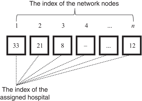
The nodes assigned to each hospital are extracted from this chromosome. The service order for the nodes assigned to a hospital is improved by a local search which applies different permutations to the service order and examines the quality of fitness function which is defined as the total number of saved patients. The best order found is returned by the local search. The capacity of each vehicle is considered equal to two patients. Furthermore, the available vehicles are randomly distributed among existing hospitals in initial solutions and it is updated through a local search which searches for best distribution of vehicles. The local search starts from a random hospital and compares the assigned vehicles to the minimum number of the vehicles required to meet its demand. If the assigned vehicles are more than the minimum requirement, the assignment is updated accordingly. The unassigned vehicles are then distributed among those hospitals whose assigned vehicles are equal or less than their minimum number of required vehicles. The minimum number of vehicles for each hospital is calculated within the fitness function.
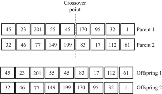
The algorithm starts with a population of random solutions. In each iteration of the GA, the offspring or children are generated by altering the selected parents through crossover and mutation operations. To perform the crossover operation, two parents are selected randomly by roulette wheel technique that gives higher priorities to better solutions with better fitness values. A unique crossover point is generated along the chromosome length, and the second part of the chromosomes after the crossover point are interchanged and two new offsprings are generated and added to the solution pool. Figure 2 depicts the crossover operation.
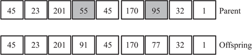
The mutation operator is performed on offspring generated by crossover operator to improve their quality. To perform mutation, one of the solutions is selected randomly. The mutation operator randomly selects some genes of the chromosome and changes the assignment of the related nodes. It should be noted that the mutation operator only applies to nodes with more than one hospital in their allowed radius, otherwise no change is possible. The mutation operation is illustrated in Figure 3.
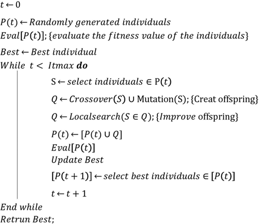
The children created by the crossover and mutation operators undergo the described local search procedures to find the best order of service for each hospital. The improved solutions are added to the population pool and the superior individuals are selected as the next generation to start the next iteration of the algorithm. The pseudo-code of the developed GA and the local searches is demonstrated in Figures 4 and 5, respectively.
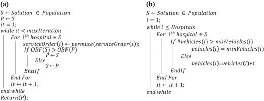
The pseudocode of (a) Local search for finding the best service order (b) Local search for finding the best assignment of vehicles
The pseudocode of (a) Local search for finding the best service order (b) Local search for finding the best assignment of vehicles
To evaluate the effectiveness of the hybrid GA with the two local searches a comparison is made between the hybrid GA and the GA. The parameters of both algorithms are tuned by Taguchi design to compare both algorithms with their best settings. The design and analysis of Taguchi are performed using Minitab 16. Taguchi reduces the number of trials by the orthogonal design of parameters (Ghadiri Nejad, Güden, Vizvári, and Vatankhah Barenji, 2018; Vatankhah Barenji et al., 2018). Thus, for the GA with four parameters and three levels, only nine runs are required. The hybrid GA with five parameters defined in three levels requires 27 runs. The Taguchi design for GA and the proposed Hybrid GA is illustrated in Table II and Table III, respectively, wherein nPop, Pc, Pm and maxIt stand for population size, crossover rate, mutation rate and the maximum number of iterations. LSI in HGA stands for the number of local search iterations. For each combination of the parameters, the algorithm is applied on three instance problems and the average value is used as the response in the analysis of the data. Considering the strategic nature of the algorithm time is not used as the response value in Taguchi analysis and only fitness values are investigated for this matter (Tables IV and V).
Taguchi design for the genetic algorithm
| nPop | Pc | Pm | maxIter | Fitness value | time |
|---|---|---|---|---|---|
| 30 | 0.5 | 0.3 | 40 | 12,749.83 | 754.52 |
| 30 | 0.6 | 0.5 | 50 | 12,781.69 | 1,355.57 |
| 30 | 0.7 | 0.7 | 70 | 12,673.66 | 2,258.48 |
| 50 | 0.5 | 0.5 | 70 | 12,730.45 | 2,189.95 |
| 50 | 0.6 | 0.7 | 40 | 12,751.85 | 2,189.95 |
| 50 | 0.7 | 0.3 | 50 | 12,693.41 | 2,348.51 |
| 70 | 0.5 | 0.7 | 50 | 12,759.88 | 2,201.78 |
| 70 | 0.6 | 0.3 | 70 | 12,703.74 | 3,806.13 |
| 70 | 0.7 | 0.5 | 40 | 12,783.75 | 3,359.79 |
Taguchi design for the hybrid genetic algorithm
| nPop | Pc | Pm | maxIt | LSI | Fitness value | time |
|---|---|---|---|---|---|---|
| 30 | 0.5 | 0.3 | 40 | 3 | 19,340.12 | 3,527.57 |
| 30 | 0.5 | 0.3 | 40 | 5 | 19,183.95 | 5,083.31 |
| 30 | 0.5 | 0.3 | 40 | 7 | 19,248.77 | 6,654.82 |
| 30 | 0.6 | 0.5 | 50 | 3 | 19,377.16 | 5,985.99 |
| 30 | 0.6 | 0.5 | 50 | 5 | 19,256.17 | 9,108.01 |
| 30 | 0.6 | 0.5 | 50 | 7 | 19,406.17 | 10,444.45 |
| 30 | 0.7 | 0.7 | 70 | 3 | 19,361.11 | 8,272.36 |
| 30 | 0.7 | 0.7 | 70 | 5 | 19,401.23 | 13,633.78 |
| 30 | 0.7 | 0.7 | 70 | 7 | 19,544.44 | 24,388.41 |
| 50 | 0.5 | 0.5 | 70 | 3 | 19,367.94 | 9,451.92 |
| 50 | 0.5 | 0.5 | 70 | 5 | 19,479.01 | 14,029.74 |
| 50 | 0.5 | 0.5 | 70 | 7 | 19,496.31 | 27,462.72 |
| 50 | 0.6 | 0.7 | 40 | 3 | 19,453.72 | 7,735.83 |
| 50 | 0.6 | 0.7 | 40 | 5 | 19,385.19 | 11,959.85 |
| 50 | 0.6 | 0.7 | 40 | 7 | 19,400.23 | 18,789.23 |
| 50 | 0.7 | 0.3 | 50 | 3 | 19,431.48 | 5,152.96 |
| 50 | 0.7 | 0.3 | 50 | 5 | 19,446.33 | 9,605.13 |
| 50 | 0.7 | 0.3 | 50 | 7 | 19,340.74 | 15,784.46 |
| 70 | 0.5 | 0.7 | 50 | 3 | 19,649.38 | 13,593.95 |
| 70 | 0.5 | 0.7 | 50 | 5 | 19,493.83 | 14,789.91 |
| 70 | 0.5 | 0.7 | 50 | 7 | 19,650.62 | 24,547.18 |
| 70 | 0.6 | 0.3 | 70 | 3 | 19,441.98 | 10,969.83 |
| 70 | 0.6 | 0.3 | 70 | 5 | 19,426.54 | 14,184.23 |
| 70 | 0.6 | 0.3 | 70 | 7 | 19,451.85 | 11,097.75 |
| 70 | 0.7 | 0.5 | 40 | 3 | 19,464.81 | 4,611.07 |
| 70 | 0.7 | 0.5 | 40 | 5 | 19,429.01 | 6,891.95 |
| 70 | 0.7 | 0.5 | 40 | 7 | 19,439.51 | 9,175.88 |
The Taguchi analysis results illustrated in Figure 6 indicates that for the GA nPop, Pc, Pm and maxIt set at 70, 0.5, 0.5 and 40, respectively, and for HGA the parameters nPop, Pc, Pm, maxIt and LSI should be set at 70, 0.5, 0.7, 50 and 7.
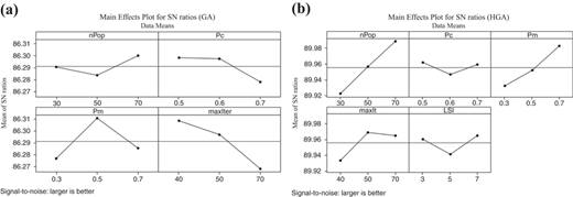
By setting the algorithms in their best configuration, algorithms were run ten times each and the results indicated in Table VI were used to compare the performance of the two algorithms. As illustrated in Table VII, the one-way ANOVA performed by Minitab software indicates that the proposed hybrid GA performs significantly better than the GA (p=0.000).
5. The case study of Tehran
5.1 The basic data of the problem
Tehran, The capital of Iran, is considered as the case study of this paper. The transportation network of this city with 90,378 nodes and 1,24,171 edges is acquired from ArcGIS. There are 235 hospitals in the city of Tehran. It is assumed there are 1,000 emergency vehicles that should be assigned to these hospitals. The average speed of the emergency vehicles is considered as 60 kilometers per hour. The place, number of accidents and the patients’ deadlines are generated randomly, and the total number of patients is equal to 45,228. The maximum, minimum, mean and standard deviation of deadlines is 80, 20, 25 and 27.95 minutes, respectively (Figure 7).
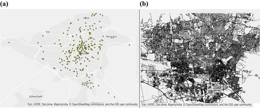
Acquired from ArcGIS (a) The hospitals of Tehran (b) Tehran transportation network
Acquired from ArcGIS (a) The hospitals of Tehran (b) Tehran transportation network
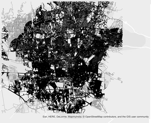
Due to the size of the problem and the high complexity and runtime required to compute the length of the shortest path between nodes, the distances between any two nodes is approximated by Manhattan distance. Furthermore, the allowable radius for assigning hospitals to nodes is set at two kilometers. This radius makes some areas out of reach. The situation is depicted in Figure 8 where reachable and unreachable areas are displayed in black and gray colors, respectively.
5.2 Results
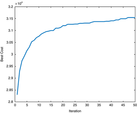
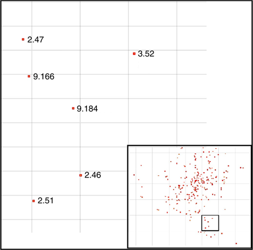
The problem under study was solved with the tuned hybrid GA with a core i5 intel computer. The number of saved people is equal to 31,541 and the CPU time for solving the problem is equal to 25076.286. These kind of algorithms are supposed to run on supercomputers which are able to process as high as 100 petaflops per seconds while the core i5 computer used for this case study can only process around 40 gigaflops per seconds (Chinese supercomputer is world’s fastest at 33,860 trillion calculations per second – Telegraph, 2013; Six Clicks: The six fastest computers in the world | ZDNet, 2017; Top 10 supercomputers of 2017 | Network World, 2017). Thus running the algorithm on a supercomputer in an emergency center would not take more than a few seconds at most. The best result acquired in each iteration of the algorithm is depicted in Figure 9. As mentioned before, the total number of patients is equal to 45,228, but only 35,344 patients have hospitals within the allowed radius. The best solution found by the algorithm with 1,000 emergency vehicles translates to saving approximately 90 percent of the patient with hospitals in their allowed radius. Furthermore the average of the deadlines is only 25 minutes which is not adequate for on time transportation, and chances of saving such patients is really low. It is needless to mention with increasing the emergency vehicles and/or the allowed radius these results may improve. The number of assigned vehicles and a corresponding number of saved patients for each hospital is illustrated in detail in Figure 10. As displayed in this figure, no vehicle is assigned to the hospitals far from the city center and most of the vehicles are in hospitals of the populated areas. The order of the service that is equivalent to the routing of the vehicles is also provided by the algorithm.
A sensitivity analysis has been carried out on the distance limit. The number of saved persons depends on the distance limit as Table VIII shows.
The number of saved persons as the function of the maximal allowed distance
| Maximal allowed distance from hospital (meter) | The number of saved persons |
|---|---|
| 1,000 | 20,320 |
| 1,500 | 29,798 |
| 2,000 | 31,541 |
| 2,500 | 28,024 |
| 3,000 | 24,663 |
| 3,500 | 22,510 |
| 4,000 | 20,568 |
As it can be seen that the maximal number of saved patients is achieved if the distance limit is 2,000 meter. The reason may be explained by the increase of traveling times resulted from the increase in allowed radius. Small radius would also put many patients out of the coverage. With the radius of 2 km, some parts of the city are not covered as it can be seen in Figure 8. The city authorities should provide required measures to overcome this problem.
The problem was solved several times without consideration of the deadlines and as expected the fatality rate was significantly higher with this policy. This result could be expected since without consideration of deadlines, a vehicle would pickup a patient with serious injury and instead of going to the nearest hospital, it would proceed to the other patient nearby, losing the chances of saving the first victim. In other case, the patients with high priority would be ignored due to their geographical location and lose their survival chance. The best rate of survival with the traditional assignment policy was 74 percent in 20 runs. These observations imply the superiority of the proposed method in terms of the saved lives which provides a better exploitation of existing resources.
There are some difficulties in deploying such a policy in real life. The main principle of the method is to serve first those with adequate deadline. The service priority is first those with shorter deadline, i.e. those with more serious injuries. In traditional policies, the emergency transportation does not differentiate between patients in such a way and such a discrimination might seem irrational to the patients and personnel. The situation is even tougher were two patients with two different priorities are near each other which would create a little conflict for those left behind or those with delayed service. However, it should be noticed the ultimate goal of disaster response is increasing the total number of saved lives and decreasing fatalities. Thus although some dissatisfaction or confusions may arise, the results are going to be significantly better. For achievement of the best results, the ERC is supposed to prioritize the patients and staff should be trained to follow the instructions strictly without deliberation. The ethical, social and legal complications encountered in this policy should be further addressed in related studies.
6. Conclusions
Even under normal situations, health cares are resource intensive units. There have been tremendous amount of studies focusing on the assignment of resources, both in terms of medical staff and medical equipment, in the various environments most of which address the post-disaster period. Maybe due to ethical issues, most of the research at hand is with the objective of maximizing the number of services, this study provides tools to optimize the number of saved lives and discusses the consequences of such decisions. It is obvious that although the number of services may be less in this strategy, the number of saved lives is greater. Investigation of ethical issues and social circumstances of such a policy is to be addressed in future studies. This paper provides disaster managers with an assignment algorithm that was not considered before.
This study applies the multiple depot pickup and delivery VRP concept for the emergency transportation of casualties of a disaster in a metropolitan city. It also uncovers some mathematical properties of the problem. The problem is known as an np-hard problem and thus a GA is devised to solve the problem. The proposed model including the proposed hybrid GA also explores which parts of the city are uncovered by the hospitals and the emergency transportation system, providing highlights for disaster management hence it also contributes to the preparedness phase.
A main aim of this study was to create a new insight into assignment of scarce medical staff to different hospitals and operating rooms to increase the success of these units in the post-disaster period. Although many relaxations were assumed in this study, the researchers hope more comprehensive models would be created in the future as a result of this study. In a post-disaster period a fleet of different aerial or ground vehicles are supposed to cooperate in emergency missions which should be captured by a fleet VRP model. The case of the post-disaster period which is a dynamic problem needs further analysis and algorithms. The last but not the least is the ethical issues associated by the method proposed which should be addressed by researchers in the field.

