


The purpose of this paper is to investigate the application of the dynamic vehicle routing problem for last mile distribution during disaster response. The authors explore a model that involves limited heterogeneous vehicles, multiple trips, locations with different accessibilities, uncertain demands, and anticipating new locations that are expected to build responsive last mile distribution systems.
The modified simulated annealing algorithm with variable neighborhood search for local search is used to solve the last mile distribution model based on the criterion of total travel time. A dynamic simulator that accommodates new requests from demand nodes and a sample average estimator was added to the framework to deal with the stochastic and dynamicity of the problem.
This study illustrates some practical complexities in last mile distribution during disaster response and shows the benefits of flexible vehicle routing by considering stochastic and dynamic situations.
This study only focuses day-to-day distribution on road/land transportation for distribution, and additional transportation modes need to be considered further.
The proposed model offers operational insights for government disaster agencies by highlighting the dynamic model concept for supporting relief distribution decisions. The result suggests that different characteristics and complexities of affected areas might require different distribution strategies.
This study modifies the concept of the truck and trailer routing problem to model locations with different accessibilities while anticipating the information gap for demand size and locations. The results show the importance of flexible distribution systems during a disaster for minimizing the disaster risks.
Nomenclature
- dod
Degree of dynamism
- E|D0|
Expected initial demand
- E|D+|
Expected additional demand
- E|Dimm|
Expected immediate demand
- di
Demand at node i
- Sets, indices, and parameters
- T
Total working hours allocated in one day
- V
A set of nodes, V={1, 2, …, |V|}
- S
A set of mini trucks available S={1, 2, …, ms}
- R
A set of trucks available R={1, 2, …, mr}
- i, j
Demand node i, j∈V
- s
Mini truck indices s∈S
- r
Truck indices r∈R
- Qs
Mini truck capacity
- Qr
Truck capacity
- tij
Travel time from node i to j
- ηj
Service time at node j
- ξi
Nonnegative stochastic (random variable) demand at node i following a normal distributionξi~N(μi,σi)
- E[ζi]
Expected demand value at node i
- γ
Demand satisfaction fraction
Continuous variables represent the capacity flow in mini truck s after serving demand node i
Continuous variables represent the capacity flow in truck r after serving demand node i
- E[FC(pr)], E[FC(ps)]
Expected additional travel time/recourse for route p by truck r and mini truck s due to capacity shortage
- Decision variables
Binary variable for truck r that travels from i to j
Binary variable for mini truck s that travels from i to j
Binary variable regarding whether node i can be serviced by truck r
Binary variable regarding whether node i can be serviced by mini truck s
1. Introduction
In the aftermath of disasters, the distribution of emergency supplies and relief goods is essential for successful disaster operations. Fast and efficient distribution systems can minimize the number of fatalities and provide quick relief to people in distress. In this regard, last mile distribution refers to the final stage of delivering relief aid from local distribution centers (LDCs) to populations in affected areas (Balcik et al., 2008), and it represents an inherent risk in the relief chain. The challenges in last mile distribution stem from the high demand for supplies due to insufficient prepositioned stockpiles, high uncertainty of actual demand, uncertainty of travel time due to infrastructure obstruction, breakdown of communication channels, transportation problems, security issues, and limited resources (Balcik and Beamon, 2008; Oloruntoba, 2010, Penna et al., 2018). Furthermore, it is common to use heterogeneous vehicles and to conduct multiple delivery trips using the same vehicle owing to an inadequate number of vehicles. In particular, the accessibility problem may result in the use of any type of “compatible” transport that is available at the time, including big trucks, vans, cars, or motorcycles.
Frequently, at the start of disaster response, sufficient information about the number of beneficiaries, exact locations, accessible routes, or quantity of relief goods required is not readily available, and specific demand is unknown. Girard et al. (2014) noted that incomplete or inaccurate information is very likely in the first five days of disaster response, during the stages from quick disaster assessment to the execution of a distribution plan. In particular, emergency services are confronted by problems such as strong dynamicity, rapid changes in data, urgency of requests, and low quality of available a priori information (Larsen and Madsen, 2000). Thus, when trying to serve all beneficiaries, continuous modification of trips becomes unavoidable. In this regard, although same-day delivery is preferred during emergencies for security reasons, doing so might not be feasible because of limited vehicle capacities or working time constraints. This consideration is a key characteristic of last mile distribution systems.
This study is motivated by the need for distributing relief goods in a time-efficient manner during disaster response. If last mile operations are executed correctly, the response time could be minimized greatly. Incorporating different types of vehicles can be beneficial to tackle issues such as accessibility or vehicle capability to reach remote and disrupted areas. However, decision makers are faced with a dynamic problem in which reliable information about victims’ locations and demands is not available, thereby forcing them to make urgent decisions with limited information and to frequently change distribution routes. To deal with this uncertainty and unpredictability, this study presents a vehicle routing model with stochastic and dynamic demand using limited heterogeneous vehicles to minimize the relief delivery time, including the expected recourse time due to demand shortage. Specifically, this study makes two main contributions. First, it develops a dynamic stochastic model using a truck and trailer routing problem (TTRP) as a humanitarian last mile distribution system. The delivery process from the LDC to demand points uses two types of vehicles to reach both accessible and nonaccessible locations. Furthermore, the concept of “information gaps” during last mile distribution is modeled as dynamic routing with stochastic demand. Second, the combination of issues faced in relief distribution at the start of disaster response, including multiple destinations, limited heterogeneous vehicles, uncertain demands and locations, and information evolution, is considered to support disaster managers’ decisions in practice.
The remainder of this study is organized as follows. Section 2 reviews relevant studies on relief distribution problems. Section 3 summarizes the problems and challenges faced in humanitarian last mile distribution systems and presents conceptual solutions and models to address them. Section 4 presents the proposed research method. Section 5 describes the numerical experiments and their results. Finally, Section 6 discusses this study’s conclusions and limitations and outlines future research directions.
2. Literature review
Quantitative methods are widely being used in operations research on disaster response operations to deal with decisions such as warehouse or distribution center locations, relief procurements, inventory, goods allocations, transportation, and relief distribution networks (Altay and Green, 2006). This paper does not review all decision models for disaster management. Instead, it specifically reviews quantitative approaches for dealing with uncertainty in relief distribution and focuses on last mile distribution planning during disaster response.
Fiedrich et al. (2000) introduced a dynamic operations model for emergency response for earthquakes and suggested an optimal assignment of resources to affected zones. Özdamar et al. (2004) investigated dynamic time-dependent distribution networks for inner-city transportation by modifying the vehicle routing problem (VRP) with pickup and delivery using multiple vehicles and commodities for minimizing unmet demand. Lin et al. (2011) developed a multiobjective mixed-integer nonlinear programming model to minimize the total unsatisfied demand, total travel time, and difference in satisfaction rate by considering the uncertainty of demand and supply. Ahmadi et al. (2015) provided a mathematical model for humanitarian logistical operations that considers road destruction possibility and standard relief time as constraints. Zhou et al. (2017) modeled dynamic resource scheduling for relief distribution in consideration of several objectives. Elluru et al. (2018) proposed a proactive and reactive model that considers both facility location and routing.
Balcik et al. (2008) noted that last mile distribution planning consists of decisions on how vehicles will make deliveries and designing the routes, including allocating relief goods to distribution centers or demand points. Yi and Kumar (2007) used an ant colony optimization (ACO) method to minimize the sum of unsatisfied demands for multicommodity relief aid while minimizing the number of unsaved people in each node. Özdamar and Demir (2012) formulated a last-mile pickup and delivery problem and proposed a hierarchical optimization model to minimize the total travel time. Noyan et al. (2014) investigated last mile distribution in post-disaster situations and proposed a two-stage stochastic model for deciding distribution locations and goods allocation to maximize the expected accessibility to distribution centers. Ahmadi et al. (2015) applied a multidepot location routing problem to last mile distribution. Ferrer et al. (2015) used the concept of vehicle routing for last mile distribution and incorporated the failure rate as reliability and security factors. Penna et al. (2018) recently used the concept of rich vehicle routing and considered accessibility constraints that allowed only compatible vehicles to serve particular routes owing to road blockage or geographical conditions.
Although many studies have investigated multitrip and heterogeneous distribution, distribution planning approaches proposed thus far have been applicable only to static planning problems. Very few studies have focused on last mile distribution with evolving and uncertain information regarding the demand size or demand location. Sheu (2010) discussed dynamic relief demand due to imperfect information and proposed the use of data fusion to forecast demand data over a period for large-scale disasters. Wohlgemuth et al. (2012) modeled the last mile distribution problem as a dynamic VRP with pickup and delivery. Lu et al. (2016) developed a real-time relief distribution model for disaster response that includes a demand and time estimator as well as a module for solving optimal distribution flows. However, most of these studies did not consider accessible or inaccessible demand locations. To the best of our knowledge, therefore, no published paper has considered both heterogeneous vehicles from an accessibility viewpoint and stochastic dynamic demand. Our study aims to address this research gap.
3. Problem description
3.1 Nature of last mile distribution
Last mile distribution in disaster response involves the distribution/movement of goods from LDCs (hubs) to beneficiaries (final delivery destinations). Last mile distribution operations are characterized by complex network designs, and therefore, several factors must be considered. From the viewpoint of the response team, one goal is that all beneficiaries should have the necessary immediate support to meet their basic needs for food and nonfood items and shelter until their permanent, long-term needs are met. However, information gaps might make it difficult to achieve this goal. Such gaps may occur when assessments leave out affected areas or groups, miscalculate actual needs due to aggregation, deal with different geographic and administrative categories resulting in data mixture, or encounter obsolete and outdated data. Each factor can be related to increased possibilities of distribution strategies, as shown in Table I.
Factors affecting last mile distribution in humanitarian logistics
| Factors | Descriptions |
|---|---|
| System description | Relief supplies from LDC to demand nodes in affected area, dynamic and stochastic environment |
| Demand location | Uncertain: a. Accessible b. Partially accessible or remote, can only be accessed by certain type of vehicle |
| Demand characterization | Uncertain, lumpy, high risk, unpredictable Multiple types: critical items at the beginning, regularly consumed item, periodically occurs |
| Vehicles | Multimodal, limited number, different compatibility with various routes |
| Route and network availability | Infrastructure limitations, damages road, nonexisted route, congestion |
| Information and decision support | Multi agents, high information gap during the beginning of operations, unreliable |
| Planning horizon | Length is variable and unknown a priori |
| Goal(s) | Varied, depending on agent/organizations, such as: maximize satisfied demand minimize response time minimize cost, etc. |
3.2 Dynamic systems and degree of dynamism (dod)
The concept of dod is used to handle the dynamic nature of and uncertainty level during the routing process. Larsen et al. (2002) defined dod as the expected percentage of uncertain requests, specifically, as the ratio between the expected number of customers at the start of the routing process and the new demand requests. The dod indicates the dynamicity of the logistics process, and the dod value decreases over time. This study uses demand-based dod, where the dynamicity is calculated by the ratio between the total immediate demand and the expected aggregate demand at the start and the expected demand deviation:
3.3 Vehicle routing plan
This section describes last mile distribution routing plans in the context of humanitarian logistics. Relief goods must be delivered from the supply side to the demand points by using available resources and infrastructure. The main task is to generate last mile distribution plans from the consolidation points or LDCs to meet the affected population within a limited amount of time. This problem is complicated by the dynamic nature of disasters and information gaps that results in dynamic distribution plans. It is also important to measure how the response to disasters must be designed to fit the characteristics of the disaster and the affected areas. In other words, humanitarian logistics should be adjustable and adaptive to respond to dynamic situations.
Given the starting point of LDCs and demand nodes, the goal of this model is to find a combination of heterogeneous vehicles to minimize the total travel time. There are two types of demand nodes in which the vehicles assigned to serve will also comply accordingly. In this model, we modify the TTRP concept to allow trucks and mini trucks to serve demand sites or LDCs, called the root of the subtour. Furthermore, mini trucks serve demands on subtours, following which they return to the root of the subtour, while trucks continue to serve remaining demands on the same route. Both vehicle types can serve independently without being limited by the same nodes.
The solution routes can be classified as follows: pure accessible routes are served by a truck (without any subtours performed by mini trucks); remote/nonaccessible routes are served by mini trucks; and partially accessible routes consisting of the main tour are traveled by trucks and at least one subtour is traveled by a mini truck. Mini trucks are used to serve demand nodes that cannot be accessed by trucks. A subtour begins and ends at the same distribution point on the main tour. In consideration of its unpredictable and unanticipated demand nodes, the route might be modified to serve new demand nodes. This modification will change the solution routes developed prior to new demand realization. Figure 1 shows dynamic routing problems for last mile distribution systems in disaster response.
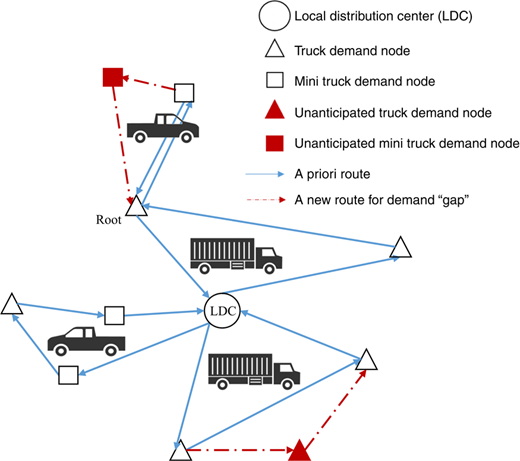
When dealing with the dynamic nature of disaster response for last mile delivery, the problem can clearly be divided into two phases based on the information quality and process evolution. First, an initial distribution plan is formulated using the limited information available for demand locations, demand volume, and infrastructure availability. Then, each vehicle is dispatched to serve the assigned route. Information gaps will inevitably result from the continuous process of modifying tours and serving demands. During emergencies, many events can impact the information available, such as infrastructure breakdowns, unsatisfied beneficiaries, additional beneficiaries from other areas, and route unavailability.
Unpredictable demand patterns and uncertain distribution routes increase the complexity of distribution plans (Balcik et al., 2008). Thus, these plans have to be modified as disaster agencies deal with such situations. By using the additional information received during the implementation of routing, the distribution plan can be modified based on the dynamics of the environment. Unlike static cases in which all customers are defined at the start of the operation, dynamic routing allows newly arriving demands to be added during routing. When a new demand is identified, operators need to decide whether to accept or reject a request. Ideally, they should be able to add unanticipated demand locations and continue with routing as per the plan. Unfortunately, this is difficult to achieve because of time constraints and vehicles’ limited capacities. Different policies are considered for allocating supplies equitably among the demands while modifying the last mile distribution network. The most recent information is observed, and unattended demands are served in the next period.
4. Methodology
4.1 Assumptions and limitations
This study postulates several assumptions and limitations to facilitate the mathematical formulation.
4.1.1 Assumptions
The set of demand nodes is divided into accessible demand nodes that can be served by both types of vehicles and nonaccessible demand nodes that can only be served by small vehicles.
Each type of vehicle has different capacities.
A set of routes is a feasible solution if the routes start and end at the LDCs. However, a subtour can start either from demand nodes (e.g. evacuation shelters, affected areas) or other designated nodes. However, the total demand for any vehicle route cannot exceed the total capacity of the allocated vehicles used in that route.
Two types of vehicles are used, and the number of vehicles required is not greater than the number of vehicles available in the fleet.
The present study focuses on the delivery of consumer goods prioritized based on urgency.
4.1.2 Limitations
The distribution plan focuses on last mile distribution, starting from LDCs to demand nodes.
Updated information regarding infrastructure, demand volume, and casualties are obtained when the first distribution/routing plan is being implemented.
This study focuses on daily-requirement demand-response goods such as water and food, and the demand volume is calculated using volume metrics.
The distribution plan is created only until all demand locations are known.
We exclude air transport and focus on road transportation.
4.2 Mathematical formulation
4.2.1 Indices, parameters, and decision variables.
Let the undirected graph G=(N, A), where N={0, 1, 2, …, n} is the set of nodes and A={(i, j): i, j∈N} is the set of links. Node 0 represents the point of distribution, and the remaining nodes in V=N⧹{0} are demand nodes. The node in which the subtour starts is called the root (c) of the main tour. A node type βi indicates whether node i can be served by a truck or a mini truck. βi=0 indicates that node i can be served by both trucks and mini trucks, and βi=1 indicates that node i can only be served by mini trucks. The nonnegative actual demand at each node i can only be known once the vehicle arrives at the demand node. K heterogeneous vehicles are available. The distribution process is only performed during working hours [0, T] for security reasons, such that each node i has available time τi∈ [0, T]. The available time indicates when both demand locations and demand amounts become known: for static demands, τi=0, and for dynamic demands, τi∈(0, T].
4.2.2 Objective function.
The objective function is to minimize the travel time, including the time needed to return to the depot or main tour route to refill the vehicle to capacity and the expected time to fulfill all demands (both priori and new demands) due to vehicle shortages:
This model is developed based on the outcome of an interview with the logistics operation manager of Badan Penanggulangan Bencana Daerah (Regional Disaster Management Agency), Yogyakarta, Indonesia, that revealed that the main concern during relief distribution is that each demand point is served (i.e. demand satisfaction). In this model, any demand gap occurrence is considered and vehicle recourse is performed given adequate working time and vehicle availability. As the model tries to satisfy all demands, the responsiveness level of the disaster response operation is optimized.
4.2.3 Constraints
Constraint (3) indicates that each demand node has to be serviced by a single mini truck or truck. Constraints (4) and (5), respectively, indicate that the mini truck and truck leave from and return to the depot and go to exactly one node. Constraints (6) and (7), respectively, express vehicle constraint flows on the routes for complete trucks and mini trucks. In the case of a disaster, limited resource availability needs to be considered. Constraints (8) and (9) ensure that at most ms mini trucks and mr trucks are used for serving nodes, respectively.
Constraints (10) and (11) express node service constraints that indicate the relationship between the binary flow variable and the binary service variable for accessible and inaccessible nodes, respectively. These constraints imply that the service variable can only be true when a vehicle physically passes a node. Constraints (12) and (13) enforce a balanced material flow requirement for demand nodes for trucks and mini trucks, respectively. However, because we have parameter ξi that represents the uncertain demand parameter, stochastic programming is needed to handle the problem of performing vehicle recourse. Real demands are unknown; however, we assume that all demands have a normal distribution with mean μi and standard deviation σi due to the deviation of demand calculation at node i. Demand deviation might occur owing to people moving from one municipal region to another or owing to incorrect calculations performed using outdated data. Constraints (14) and (15) express the construction of demand flows as long as sufficient capacity is available. It should be noted that travel times vary depending on road conditions, traffic conditions, or vehicle speed, especially during disaster response.
However, we limit this study to considering only deterministic time. We realize that distributing goods during nighttime will not be feasible owing to security reasons. Thus, additional constraints regarding time are added. Constraints (16) and (17) indicate that the total service time for each vehicle type cannot exceed the available distribution time. Finally, constraints (18) and (19) impose domain conditions on the variables.
4.3 Routing policies: recourse function and dynamic demand allocation
4.3.1 Initial solution for vehicle route.
We illustrate the effects of different demand node types, demand amounts, and network characteristics on vehicle allocation and route planning. The model assumes that one demand node can only be visited one time during one working period, with a limited number of available vehicles. Assuming vehicle capacity Qr=300 and Qs=150, Figure 2 shows the routing and vehicle allocation decision for five demand nodes, one LDC node, and four available vehicles (ms=2, mr=2) in the initial distribution planning phase. The distribution should be planned based on vehicle availability, vehicle capacity, and allowable time constraints. Thus, the initial solution ensures route feasibility based on the following equations:
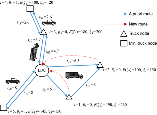
Example of allocation of four available vehicles for one LDC and five demand nodes
Example of allocation of four available vehicles for one LDC and five demand nodes
Both equations guarantee that the expected total demand does not exceed the respective vehicle capacities. All constructed routes satisfy the conditions specified by the constraints, and the total times for all routes are minimized using ∑t=48.1. In addition, when the route needs to be modified owing to the probability of shortage, a recourse can be factored in to serve the next customer. Therefore, the first route is modified by considering the possibility of shortage, in addition to other constraints such as vehicle capacity and availability of working time. This results in additional recourse time △t=5.5 compared to no recourse. As a tradeoff, all demands can be satisfied.
4.3.2 Vehicle recourse function in shortage situations.
Route failure occurs when a vehicle is running out of capacity and is therefore not able to fully service current customer i or when the distribution process exceeds its working time T. The first case occurs because there is a probability that the remaining vehicle capacity will not be enough to satisfy the demand for the next node; as a result, the current route is terminated. The second case occurs if there is road blockage or traffic congestion during the distribution process. This subsection focuses on the first case where failure occurs owing to a shortage of supplies.
After a vehicle is dispatched, at each node it services, the probability of shortage for the next node is calculated. If the probability is higher than the level of confidence, recourse will need to be taken. The probability of the cumulative demand up to customer i is calculated by following the recursive concept proposed by Gendreau et al. (1996). Following the recourse action, which consists of sending the vehicle back to the depot, notifying the depot to send another vehicle (if available), or replenishing the same vehicle to serve again, the vehicle continues to serve customer i and resumes the route as originally planned. If recourse is performed, additional travel time must be added to account for the vehicle’s return to the LDC for replenishing supplies. However, this policy requires a feasibility check of the maximum working hours, because recourse implies additional time. However, in light of multimodal vehicles and subtour formations, recourse might occur from a node in the subtour to the root of the main tour. Thus, five types of recourse functions are considered.
Given a route p (i1, i2, …, ih), where il∈V for h∈{1, 2, …, h}, the cumulative expected demand at ih will be with expected cumulative variance equal to . The expected failure cost/recourse function at demand node ih for p is . Notation u denotes when failure occurs at ih given that it has not occurred on any previously visited customer along the route. The detailed calculation for each recourse type is as follows:
Failure occurs in nonaccessible route served by mini truck.
This failure occurs if the cumulative demand up to customer ih is larger than the mini truck capacity . In nonaccessible routes, the vehicle will return to depot (0) to refill supplies and continue to service the demand from ih according to the following equation:
(22)Failure occurs in subtour of partially accessible route served by mini truck.
If occurs in the subtour of a partially accessible route, then the vehicle will return to the root (r) of the main tour, refill supplies, and continue to service the demand from ih according to the following equation:
(23)Failure occurs in pure accessible route served by truck.
This failure occurs if the cumulative demand up to customer ih is larger than the truck capacity :
(24)Failure occurs in partially accessible route served by truck after servicing the subtour.
In this case, the truck capacity is Qr−Qs as the subtour has been serviced. Thus, failure will occur if the cumulative demand up to customer ih is larger than the available truck capacity :
(25)Failure occurs in any tour with cumulative demand up to customer ih equal to vehicle capacity.
If is equal to vehicle capacity, then after the vehicle refills supplies (either at depot (0) or root (c) of main tour), it will continue the service from ih+1 according to the equations for mini trucks and trucks, respectively:
(26)(27)
4.3.3 Dynamic demand allocation.
Unlike in static cases where all customers are defined at the start of operations, dynamic routing involves newly arriving demands n+ during routing hours. Thus, assuming that n+ demand nodes are added, let the new customer set V+={n+1, n+2, …, n+n+}. The set of all demand nodes will be V′=V∪V+ for all locations N′=V′∪{0}, with the travel times between i and j for all i, j∈N′ denoted as tij.
For meeting the requirements of dynamic demand, we model the problem as a sequence of static subproblems. The distribution horizon T is split into s parts, such that the time interval for each part is v=T/s. When a new demand is identified, the vehicle needs to decide whether to accept or reject the request based on the availability of relief goods and time. When the dynamic demand is known in τi∈(0, T], the vehicle needs to check the availability of supplies, probability of shortage, and vacant time. If all conditions are satisfied, then the new demand can be added to the route; otherwise, it shifts to the next working slot. All these dynamics nodes are treated as static customers for the next distribution period.
4.4 Solution method
4.4.1 Simulated annealing (SA)/variable neighborhood search (VNS).
Gendreau et al. (2001) suggested that a metaheuristic approach is suitable for major class optimization problems such as the VRP and its variants. Neighborhood-centered methods generally proceed by iteratively exploring the neighborhoods of a single incumbent solution; examples of such methods include SA (Kirkpatrick et al., 1983), Tabu search (Glover and Laguna, 2013; Taillard, 1993), VNS (Mladenovic and Hansen, 1997; Kytöjoki et al., 2007), adaptive large neighborhood search (ALNS) (Ropke and Pisinger, 2006), and iterated local search (ILS) (Lourenço et al., 2003). By contrast, population-based methods are inspired by natural mechanisms; examples of such methods include genetic algorithms (GA) and evolutionary algorithms (EA) (Holland, 1975), memetic algorithm (Moscato and Cotta, 2010), path relinking, scatter search (Glover, 1999), particle swarm optimization (Eberhart and Kennedy, 1995), and ACO (Dorigo and Stützle, 2003). Numerous types of hybrid metaheuristics have also been proposed for solving VRP variants; these include SA+Tabu (Osman, 1993), greedy randomized adaptive search procedure (GRASP)+ILS (Prins, 2009), ILS+variable neighborhood descent (VND) (Chen et al., 2010), and TABU+ILS (Cordeau and Maischberger, 2012).
Single-solution-based heuristics have been extensively studied because of their proven ability to solve NP-hard problems with robust quality and time efficiency. TTRP, a VRP variant, is one such problem that can be solved effectively using this approach. Some notable methodologies include Tabu search (Chao, 2002; Scheuerer, 2006), SA (Lin et al., 2009), large neighborhood search (Derigs et al., 2013), hybrid GRASP (Villegas et al., 2010, 2011), and matheuristic (Villegas et al., 2013; Drexl, 2011). Furthermore, some methods such as VNS (Gutjahr et al., 2007; Sarasola et al., 2016), ALNS (Azi et al., 2012), and hybrid metaheuristics (Ritzinger, and Puchinger, 2013) have been shown to provide robust results for solving both stochastic and dynamic VRP variants. Many researchers have proposed metaheuristics approaches for solving disaster response problems. For example, Yi and Kumar (2007) used ACO, Lin et al. (2011) used GA, Wilson et al. (2013) used VND, and Zhou et al. (2017) used EA.
Heuristic algorithms are more popular than exact approaches for solving mathematical models with high complexity. Thus, this study proposes the use of a hybrid SA algorithm that can use a hill-climbing approach to escape from local optima (Gendreau and Potvin, 2010). We modified the basic SA algorithm to solve dynamic stochastic problems. The SA algorithm itself comprises two stochastic processes, one of which is the solution acceptance criterion; therefore, it does not require any modifications for solving stochastic problems. An event scheduler architecture developed by Montemanni et al. (2005) is used to deal with dynamic demand requests with the timestamp. However, it is also important to note that the initial solution and intensification phase of the algorithm affect the quality of the ultimate solution. Furthermore, as we add VNS to the diversification and intensification strategy, we include the stochastic framework by adding the sample average estimator (SAE) that is performed if a comparison is required during the MoveorNotMove part.
The proposed SA algorithm has been successfully applied to a combinatorial optimization problem such as VRP and its variants, such as TTRP. Its probabilistic mechanism, which is based on the Monte Carlo simulation, can easily capture the uncertainty and randomness of disaster response operations. Furthermore, it can be combined with other methods and can be modified and hybridized easily, thus strengthening its ability to deal with complex real-world disaster response problems. Many studies have successfully applied SA algorithms to various problems, and therefore, this study uses a hybrid SA/VNS approach.
4.4.2 Initial solution.
The solution is represented by a permutation of n customers denoted by a set of string numbers {1, 2, 3, …, n}. Additional zeros are added to represent LCDs and points for subtours. Each demand number has additional information regarding the types of demands/services that indicate that the node is served by a particular vehicle on a different route. We use two types of initial solutions, namely, ISG and ISN:
Heuristic initial solution (ISG): it is important to allocate demand nodes to the routes associated with their types of demand. Thus, this study adopted and incorporated the generalized assignment problem (GAP) to solve the node allocation problem (refer to Chao, 2002 for the detailed algorithm). After all demand nodes are allocated to a particular route, the demand node sequence problem for each route is constructed using the insertion heuristic.
Nearest neighbor (ISN): by using the GAP concept for node allocation, path construction is performed using information relay based on nearest neighborhood heuristics. We try to find the closest candidate node with respect to travel time t. As we deal with multimodal routing and subtours are allowed, it is necessary to modify the basic nearest neighbor. First, we consider a number of unimodal graphs {G1, G2, G3} that represent each vehicle associated with different types of routes. Each graph consists of nodes, arcs, and demand label sets Gi=(Vi, Ai, Li). The arc set is the union of all input graphs’ arcs and a set of transfer arcs Atransfer; therefore, the total arc set is Amm=A1∪A2∪A3∪Atransfer. Transfer arcs are used to connect the unimodal graphs, and they make it possible to transfer from one unimodal graph to another.
4.4.3 Detailed algorithm.
Because the problem is a mix of stochastic and dynamic routing problems, it is important to treat it as a multitime interval static problem. Then, a plan must be formulated at the start of each time interval for how to service the currently known demand nodes. Recourse will be considered at the same time if the constraints are satisfied. Otherwise, the plan will be changed at the start of the next time interval. In dynamic problems, it is important to embed the simulator that will receive new demand requests and manage the simulation time Tsim such that when the dynamic demand is known in τi∈(0, T], the vehicle will try to service the demand as soon as possible or process it at the end of the time period. As explained in Section 4.3.3, the distribution horizon T is split into s parts with v time intervals. First, the event scheduler sets the simulation time, and then, the initial solution is constructed based on static demand node information (Section 4.4.2). Optimization is performed until the current T/s is over and the vehicle is sent to new demand nodes in the next T/s time units. In the following periods, this process is repeated using the solution from the previous period and by including new demand nodes using the Clarke-Wright algorithm (Clarke and Wright, 1964).
The SA/VNS optimization for each timestamp v will improve the results of the initial solution by randomly choosing different improvement moves, such as swap, insertion, 2-opt, and reverse. We also allow a change in service vehicle type for obtaining more diverse solutions by exchanging the vehicles used in particular nodes as long as the solution is feasible. The algorithm starts by setting current temperature Temp0 and generating an initial solution X. The current best solution Xbest and the best objective function of X Fbest are set to X and obj(X)), respectively. Figure 3 shows a flowchart of the SA/VNS algorithm.
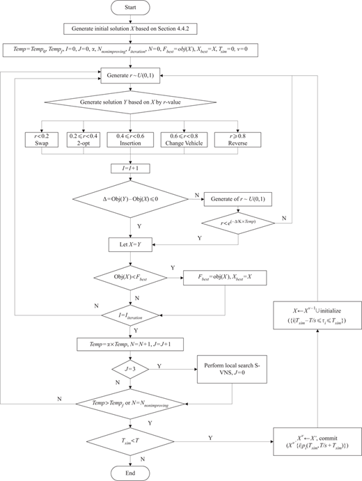
For diversification and intensification, we use the stochastic variable neighborhood search (S-VNS) algorithm. This local search is performed after every three temperature Temp decrements. The SAE procedure is performed in VNS to use stochastic information to compare solutions. The procedure draws a sample of scenarios of unserved customer demands to obtain the average value of objectives function in each scenario. However, we select different types of neighborhoods in the VNS algorithm. First, we adopt subtour removal heuristics that relocate subtours and transfer them to other potential roots. The other neighborhoods are 2-opt and 2opt*.
5. Results and discussions
The proposed SA/VNS was implemented in Microsoft Visual C++ 2012 and executed on a computer with an Intel i5 2.66 GHz CPU and 16 GB RAM running the Windows 7 64-bit operating system. The proposed method was first tested on Chao’s (2002) TTRP benchmark that consisted of 21 instances of 50-199 demand nodes to understand its performance. Then, the proposed algorithm was used to solve the problem derived from a real case study in Yogyakarta, Indonesia. The experiment compared the performance of the SA/VNS implementation using basic SA, SA/VNS-ISG, and SA/VNS-ISN.
This study uses Taguchi’s method with a two-level factorial design to set parameters. The result of this design experiment indicates that the best parameter combination for SA is Nnonimproving=2N, initial temperature T0=1, final temperature Tf=0.01, number of iterations Iiteration=500×N, Boltzmann constant K=1/3, and cooling coefficient α=0.9, where N is the total number of demand nodes. We also performed an analysis to determine the maximum number of neighborhoods (kmax) in the VNS algorithm, and we set kmax=3 to reduce the computational time.
5.1 Algorithm verification
To benchmark the performance of the proposed SA/VNS algorithm, we compared it with other methods. We used 21 instances from Chao’s (2002) data sets and compared it with best-known solution (BKS). The data set comprised seven sizes with 50-199 demand nodes and three different proportions of node types, namely, 25, 50, and 75 percent. All three modifications of the proposed algorithm were run ten times, and the best solution was recorded. The algorithm’s performance was measured in terms of the percentage gap between the algorithm’s solution values and the BKS values by considering the average performance of the algorithm. As the data sets were deterministic with static demand, we did not use the demand simulator to run the instances; instead, we focused on minimizing the distances traveled by vehicles.
As shown in Table II, the basic SA/VNS algorithm with random initial solutions performed well in medium-sized instances with 50-75 demand nodes. However, we failed to achieve optimal results for instances with more than 75 nodes. In contrast, the modified SA/VNS with ISN and ISG could solve instances with up to 120 demand nodes. However, it still failed to reach the best-known solutions for instances with more demand nodes. The modified SA/VNS with ISN and ISG obtained 11 and 13 BKSs out of 21 data sets and registered average deviations from the BKS of 0.16 and 0.11 percent, respectively. The results for both modified SA/VNS algorithms deviate at most within 1.03 and 0.66 percent from the BKS. Although SA/VNS-ISG seems to show a better result than SA/VNS-ISN, the difference is not significant considering that the p-value of the statistical test is 0.35304008, which is greater than the α(0.05) value, indicating no significant difference between the results obtained by SA/VNS-ISG and SA/VNS-ISN.
Comparison with a state-of-the-art method for the deterministic TTRP
| Data set | Node | Best-known solution (BKS) | SA/VNS | Gap (%) | SA/VNS-ISN | Gap (%) | SA/VNS-ISG | Gap (%) |
|---|---|---|---|---|---|---|---|---|
| 1 | 50 | 564.68a | 564.68 | 0.00 | 564.68 | 0.00 | 564.68 | 0.00 |
| 2 | 611.53b | 611.53 | 0.00 | 611.53 | 0.00 | 611.53 | 0.00 | |
| 3 | 618.04a | 618.04 | 0.00 | 618.04 | 0.00 | 618.04 | 0.00 | |
| 4 | 75 | 798.53a | 808.84 | 1.29 | 798.53 | 0.00 | 798.53 | 0.00 |
| 5 | 839.62a | 839.62 | 0.00 | 839.62 | 0.00 | 839.62 | 0.00 | |
| 6 | 930.64b | 930.64 | 0.00 | 930.64 | 0.00 | 930.64 | 0.00 | |
| 7 | 100 | 830.48a | 830.48 | 0.00 | 830.48 | 0.00 | 830.48 | 0.00 |
| 8 | 870.94c | 875.76 | 0.55 | 872.56 | 0.19 | 872.56 | 0.19 | |
| 9 | 912.02b | 912.64 | 0.07 | 912.02 | 0.00 | 912.02 | 0.00 | |
| 10 | 150 | 1,036.2e | 1,053.9 | 1.71 | 1,039.07 | 0.28 | 1,039.07 | 0.28 |
| 11 | 1,091.9c | 1,093.57 | 0.15 | 1,093.57 | 0.15 | 1,091.9 | 0.00 | |
| 12 | 1,149.4c | 1,155.44 | 0.52 | 1,154.7 | 0.46 | 1,154.7 | 0.46 | |
| 13 | 199 | 1,284.7c | 1,320.21 | 2.76 | 1,287.1 | 0.19 | 1,287.1 | 0.19 |
| 14 | 1,333.7c | 1,351.54 | 1.34 | 1,347.4 | 1.03 | 1,333.7 | 0.00 | |
| 15 | 1,416.5c | 1,436.78 | 1.43 | 1,425.8 | 0.66 | 1,425.8 | 0.66 | |
| 16 | 120 | 1,000.8e | 1,004.47 | 0.36 | 1,002.4 | 0.16 | 1,004.47 | 0.36 |
| 17 | 1,026.2d | 1,026.88 | 0.07 | 1,026.2 | 0.00 | 1,026.2 | 0.00 | |
| 18 | 1,098.2d | 1,099.09 | 0.09 | 1,098.2 | 0.00 | 1,098.2 | 0.00 | |
| 19 | 100 | 812.69d | 814.07 | 0.17 | 813.3 | 0.08 | 813.3 | 0.08 |
| 20 | 848.12e | 855.14 | 0.83 | 848.93 | 0.10 | 848.93 | 0.10 | |
| 21 | 909.06a | 909.06 | 0.00 | 909.06 | 0.00 | 909.06 | 0.00 | |
| Average gap (%) | 0.54 | 0.16 | 0.11 | |||||
| Number of BKS | 7 | 11 | 13 |
Note: Italics values indicate that the BKS has been found
Both of our SA/VNS heuristics can solve the TTRP in terms of solution quality. Therefore, the analyses indicate that to obtain quality solutions for the TTRP, the proposed SA/VNS heuristic is as effective as other heuristics and seems to be as efficient. However, it failed to outperform the solution quality of matheuristics. In particular, the proposed algorithms achieved the best results in small and medium instances with up to 75 demand nodes.
5.2 Case study and data sets
5.2.1 Case study description.
In 2006, a powerful Mw 5.9 earthquake struck Yogyakarta, Indonesia, causing more than 5,000 deaths and destroying 370,776 private houses and public structures (BAPPENAS, 2006). A field study and data collection drive conducted in 2016 in Yogyakarta, Indonesia, revealed that although the Badan Penanggulangan Bencana Daerah (Regional Disaster Management Agency), Yogyakarta, is currently very actively coordinating with local and international nongovernmental organizations’ disaster risk reduction projects, there unfortunately remains a great lack of awareness about the importance of relief supply chains and their preparedness.
Owing to inadequate information about evacuation processes, including where to evacuate temporarily, earthquake victims scattered over a large area in relatively small groups and frequently moved to look for safer places or relief aids. These problems hampered the disaster response teams, as the exact information kept changing and became unreliable, resulting in deviations in the actual demand volume and location accuracy.
This section discusses the applicability of the proposed dynamic model for last mile distribution by considering different types of demand nodes and limited vehicle availability. In commercial logistics, demand data can be forecasted, and demand error can be corrected easily. However, logistics management in disaster situations relies entirely on administrative data held by the government, which leads to the need for flexible relief distribution. Accordingly, this study uses past data in the numerical analysis to show the model’s performance over a set of more realistic data.
5.2.2 Data sets.
All 17 wards in Bantul District, Yogyakarta, Indonesia, were chosen to test the model and calculations. Each ward has a different topography and has different proportions of low- and high-accessibility demand nodes. The number of initial demand points is based on the number of villages/hutments in each ward, and the locations are scattered. The LDC is located within the ward boundary. Table III shows the demand data for the ward.
Details of the demand data set
| Data set | Ward name | Initial number of demand points | Total population in need of relief | Demand node proportion (low accessibility:high accessibility) |
|---|---|---|---|---|
| B_01 | Bantul | 50 | 58,462 | 10:90 |
| B_02 | Dlingo | 58 | 34,263 | 60:40 |
| B_03 | Imogiri | 72 | 56,446 | 50:50 |
| B_04 | Jetis | 64 | 50,974 | 20:80 |
| B_05 | Pundong | 49 | 31,447 | 30:70 |
| B_06 | Banguntapan | 57 | 98,557 | 15:85 |
| B_07 | Bambang Lipuro | 45 | 38,223 | 30:70 |
| B_08 | Kasihan | 53 | 92,099 | 25:75 |
| B_09 | Kretek | 52 | 28,648 | 40:60 |
| B_10 | Pajangan | 55 | 28,942 | 40:60 |
| B_11 | Pandak | 49 | 45,924 | 50:50 |
| B_12 | Piyungan | 60 | 44,811 | 20:80 |
| B_13 | Pleret | 47 | 41,902 | 25:75 |
| B_14 | Sanden | 62 | 29,449 | 25:75 |
| B_15 | Sedayu | 54 | 40,948 | 30:70 |
| B_16 | Sewon | 63 | 87,786 | 25:75 |
| B_17 | Srandakan | 43 | 28,367 | 75:25 |
The requirement for relief goods was calculated based on the standard requirements established by the disaster agency in Indonesia (Badan Nasional Penganggulangan Bencana, 2009). According to the disaster agency, the basic consumable goods needed by one person per week are as follows:
Rice: 2.8 kg/week.
Drinking water: 15-20 L/week.
Supplementary foods: 1.2 kg/week.
Others: 0.5 kg/week.
Accordingly, the amount of relief goods needed was calculated by multiplying the basic needs for one person/week and the population count in each demand node. Considering that water occupies more space based on its demand, we divided the vehicles into those that would transport water and those that would transport foods. However, the distribution followed the same route with the assumption that both goods would be transported at the same time. The travel time was calculated based on the travel distance divided by the worst-case speed during the distribution process (e.g. 30 km/hour).
5.3 Computational results and discussion
Solutions were provided for a total of 17 case studies, one for each ward in Bantul, Yogyakarta, using four different algorithms, namely, SA, VNS, ACO, and our proposed hybrid SA/VNS. We compared the results from the computational experiments to determine the performance of our proposed algorithm. In this section, we compare basic SA and VNS to understand the robustness of our hybrid algorithm compared to the basic algorithm. We also compare it with ACO, a population-based algorithm that can solve VRP variants; the results are competitive, although the computational time is slightly longer (Yu et al., 2009). As there are two types of initial solutions, as stated in Section 4.4.2, the best result from between the two hybrid methods, namely, SA/VNS-ISN and SA/VNS-ISG, is selected. For all cases, we first ran the deterministic problem as an initial distribution plan. Then, we ran the dynamic stochastic problem with default settings that included 10 percent dod and 10 percent demand standard deviation from the initial data stated in Table IV. In this computational experiment, we set the number for each vehicle type as 20 with the following specifications: mini trucks have 20-ton capacity and trucks have 30-ton capacity. Table IV shows the computational results in terms of distance travel and computational time for stochastic dynamic routing.
Dynamic stochastic result comparison with several algorithms
| SA | VNS | ACO | SA/VNS | |||||
|---|---|---|---|---|---|---|---|---|
| Data set | Travel distance | Time (seconds) | Travel distance | Time (seconds) | Travel distance | Time (seconds) | Travel distance | Time (seconds) |
| B_01 | 2,072.63 | 173.84 | 2,148.27 | 165.37 | 2,072.63 | 261.94 | 2,072.63 | 170.71 |
| B_02 | 1,783.16 | 141.67 | 1,754.78 | 101.40 | 1,717.07 | 200.01 | 1,682.30 | 178.32 |
| B_03 | 3,914.25 | 163.40 | 3,831.12 | 144.99 | 3,739.80 | 370.41 | 3,609.62 | 223.71 |
| B_04 | 2,616.33 | 175.89 | 2,583.98 | 179.00 | 2,501.28 | 354.53 | 2,513.26 | 235.48 |
| B_05 | 1,818.63 | 136.12 | 1,782.92 | 127.23 | 1,782.92 | 145.02 | 1,782.92 | 138.23 |
| B_06 | 3,619.78 | 160.99 | 3,619.78 | 123.77 | 3,336.65 | 253.26 | 2,957.47 | 179.20 |
| B_07 | 1,515.08 | 128.58 | 1,591.65 | 98.23 | 1,477.72 | 117.07 | 1,515.08 | 130.97 |
| B_08 | 2,964.94 | 175.89 | 2,973.20 | 129.00 | 2,843.14 | 233.39 | 2,843.14 | 181.33 |
| B_09 | 1,910.06 | 129.63 | 1,809.57 | 111.09 | 1,822.27 | 232.08 | 1,809.57 | 138.05 |
| B_10 | 1,683.74 | 156.38 | 1,683.74 | 171.44 | 1,612.16 | 288.13 | 1,531.46 | 168.61 |
| B_11 | 2,002.66 | 127.30 | 2,002.66 | 108.72 | 1,987.71 | 197.83 | 1,982.31 | 124.30 |
| B_12 | 2,155.08 | 153.67 | 2,196.40 | 129.48 | 1,894.01 | 280.69 | 1,894.01 | 185.95 |
| B_13 | 1,580.29 | 110.81 | 1,705.39 | 99.31 | 1,580.29 | 160.99 | 1,580.29 | 132.87 |
| B_14 | 1,809.71 | 152.63 | 1,856.82 | 149.49 | 1,809.71 | 349.04 | 1,762.05 | 162.10 |
| B_15 | 1,864.89 | 153.67 | 1,864.89 | 113.95 | 1,807.87 | 277.98 | 1,810.20 | 150.15 |
| B_16 | 2,757.19 | 177.72 | 2,834.49 | 110.81 | 2,757.19 | 302.33 | 2,693.96 | 195.49 |
| B_17 | 1,504.79 | 100.56 | 1,452.76 | 94.08 | 1,487.36 | 142.17 | 1,452.76 | 125.78 |
| Average | 2,210.19 | 148.16 | 2,217.20 | 126.90 | 2,131.16 | 245.11 | 2,087.83 | 165.96 |
| Number of Best solution found | 2 | 3 | 8 | 14 | ||||
Note: Italics values indicate the best solution found during the computational experiment
Table IV shows that the proposed SA/VNS provides better results in terms of solution quality compared to the other algorithms. Italic numbers indicate that the objective function value is equal to the best solution found during the computational experiment. The result in Table V shows that the solution quality of the ACO result is better than that of the basic SA or VNS results. However, SA/VNS shows a slightly better result compared to ACO. SA/VNS can achieve 14 better solutions compared to other algorithms, and ACO can also provide better solutions compared to SA or VNS. Specifically, for data B_04, B_07, and B_15, ACO outperforms our proposed algorithm with a slightly better result. ACO performs well when the number of inaccessible nodes is less than 40 percent regardless of the total number of demand locations that need to be served. This may be because ants (on whom ACO is based) choose a route based on either its attractiveness (i.e. travel distance) or pheromone level (that indicates past movement). The additional information relay for each time interval might help to improve the ACO performance.
Dynamic stochastic result for 17 wards in Bantul district using two types of proposed algorithm
| SA/VNS-ISN (1) | SA/VNS-ISG(2) | |||||||||
|---|---|---|---|---|---|---|---|---|---|---|
| Initial solution | Dynamic routing | Initial solution | Dynamic routing | Travel time gap ((1)−(2)/(1)) | ||||||
| Data set | Travel distance (km) | Travel time (hours) | Travel distance (km) | Travel time (hours) | Travel distance (km) | Travel time (hours) | Travel distance (km) | Travel time (hours) | Initial solution(%) | Dynamic routing(%) |
| B_01 | 1,632.52 | 54.42 | 2,155.65 | 71.86 | 1,632.52 | 54.42 | 2,072.63 | 69.09 | 0.00 | 3.85 |
| B_02 | 1,375.22 | 45.84 | 1,682.30 | 56.08 | 1,370.73 | 45.69 | 1,783.16 | 59.44 | 0.33 | −6.00 |
| B_03 | 2,642.75 | 88.09 | 3,609.62 | 120.32 | 2,617.42 | 87.25 | 3,739.80 | 124.66 | 0.96 | −3.61 |
| B_04 | 1,701.03 | 56.70 | 2,513.26 | 83.78 | 1,700.89 | 56.70 | 2,532.74 | 84.42 | 0.01 | −0.78 |
| B_05 | 1,369.28 | 45.64 | 1,782.92 | 59.43 | 1,369.28 | 45.64 | 1,916.71 | 63.89 | 0.00 | −7.50 |
| B_06 | 2,250.72 | 75.02 | 2,957.47 | 98.58 | 2,250.72 | 75.02 | 2,970.28 | 99.01 | 0.00 | −0.43 |
| B_07 | 1,242.51 | 41.42 | 1,838.51 | 61.28 | 1,243.09 | 41.44 | 1,515.08 | 50.50 | −0.05 | 17.59 |
| B_08 | 2,370.57 | 79.02 | 3,205.64 | 106.85 | 2,370.57 | 79.02 | 2,843.14 | 98.83 | 0.00 | 7.51 |
| B_09 | 1,319.35 | 43.98 | 1,809.57 | 60.32 | 1,319.22 | 43.97 | 1,817.11 | 60.57 | 0.01 | −0.42 |
| B_10 | 1,226.67 | 40.89 | 1,531.46 | 51.05 | 1,228.25 | 40.94 | 1,682.42 | 58.08 | −0.13 | −9.68 |
| B_11 | 1,528.17 | 50.94 | 1,982.31 | 66.08 | 1,528.03 | 50.93 | 2,021.84 | 67.39 | 0.01 | −1.99 |
| B_12 | 1,527.65 | 50.92 | 2,529.92 | 84.33 | 1,526.66 | 50.89 | 1,894.01 | 63.13 | 0.06 | 25.14 |
| B_13 | 1,342.89 | 44.76 | 1,865.40 | 62.18 | 1,342.89 | 44.76 | 1,580.29 | 52.68 | 0.00 | 15.28 |
| B_14 | 1,310.64 | 43.69 | 1,951.85 | 65.06 | 1,315.59 | 43.85 | 1,762.05 | 58.74 | −0.38 | 9.72 |
| B_15 | 1,416.91 | 47.23 | 1,947.41 | 64.91 | 1,416.86 | 47.23 | 1,810.20 | 60.34 | 0.00 | 7.05 |
| B_16 | 2,218.37 | 73.95 | 3,128.24 | 104.27 | 2,214.09 | 73.80 | 2,693.96 | 89.80 | 0.19 | 13.88 |
| B_17 | 1,183.15 | 39.44 | 1,452.76 | 48.43 | 1,182.81 | 39.43 | 1,605.82 | 53.53 | 0.03 | −10.54 |
| Average | 0.06 | 3.47 | ||||||||
Note: Italic values indicate a higher quality solution
In terms of computational time, VNS is slightly faster compared to SA and hybrid SA/VNS. By contrast, ACO is slower compared to SA, VNS, and SA/VNS, as has been mentioned previously (Yu et al., 2009). Although SA and VNS have low computational time, their solution quality gap with SA/VNS is 5.86 and 6.19 percent, respectively. SA/VNS combines the complexity of the local search implementation by using VNS, which requires slightly longer computational time. Nevertheless, SA/VNS has a reasonable computational time and provides a robust result.
As the proposed algorithm can solve the problem with better results, its results are discussed in detail. Table V shows the results of the proposed methods for solving deterministic and stochastic dynamic distribution plan problems. For the 17 data sets solved, SA/VNS-ISG seems to perform slightly better in terms of average gap for initial and dynamic routing phases. However, both proposed algorithms show varied performance in terms of solution quality for each data set. In the initial solution phase, SA/VNS-ISN tends to show better results for smaller population data sets, which also have mostly accessible demand nodes available. By contrast, SA/VNS-ISG performs better for a relatively higher number of less-accessible demand nodes.
However, after stochastic data and dynamic requests were obtained, the performance of both algorithms changed slightly. SA/VNS-ISG showed better solution quality for data sets that had a higher proportion of accessible demand nodes, whereas SA/VNS-ISN showed the opposite tendency. We performed a t-test with α=0.05 for both solutions (initial and dynamic phase) and found that the difference is not significant for both cases, with p-values of 0.293 and 0.271 for the initial and dynamic phase, respectively. We suggest that although the nearest neighbor seems to be less robust in deterministic cases, it fits with stochastic and dynamic cases as it offers a higher possibility to include or modify the route during the modification process in cases when the demand proportion of less-accessible demand nodes is higher.
Table VI shows the required number of vehicles for distribution planning and additional travel time as result of route modification. The total number of vehicles is linearly proportion to the relief goods needed, with data sets B_06, B_08, and B_16 requiring the most vehicles. As the vehicles have limited capacities, additional demand forces the use of additional vehicles for completing the distribution. On average, the number of mini trucks and trucks increased by 11 percent (~1 vehicle) and 16 percent (~1 vehicle), respectively. Our statistical test shows the increase in the number of mini trucks with p-value <α(0.05), as shown in Table VII. However, the number of trucks used does not significantly increase after the dynamic phase with p-value >α(0.05), as also shown in Table VII. As many data sets have a significant proportion of less-accessible nodes, the number of mini trucks used in distribution routing is higher than the number of trucks. Although mini trucks have smaller capacity, using mini trucks from the start provides advantages during distribution, such as not requiring a change in vehicle type and the ability to be used for all types of demand nodes.
Number of vehicles used
| SA/VNS-ISN (1) | SA/VNS-ISG(2) | |||||||||
|---|---|---|---|---|---|---|---|---|---|---|
| Initial solution | Dynamic routing | Initial solution | Dynamic routing | |||||||
| Data set | Mini truck | Truck | Mini truck | Truck | Additional travel time (hours) | Mini truck | Truck | Mini truck | Truck | Additional travel time (hours) |
| B_01 | 9 | 8 | 10 | 9 | 17.44 | 9 | 8 | 10 | 9 | 14.67 |
| B_02 | 7 | 1 | 7 | 2 | 10.24 | 7 | 1 | 7 | 2 | 13.75 |
| B_03 | 9 | 6 | 10 | 7 | 32.23 | 9 | 7 | 10 | 7 | 37.41 |
| B_04 | 9 | 8 | 10 | 10 | 27.07 | 9 | 8 | 10 | 9 | 27.73 |
| B_05 | 6 | 3 | 7 | 3 | 13.79 | 6 | 3 | 7 | 3 | 18.25 |
| B_06 | 15 | 15 | 17 | 15 | 23.56 | 15 | 15 | 18 | 15 | 23.99 |
| B_07 | 6 | 5 | 8 | 4 | 19.87 | 6 | 5 | 7 | 6 | 9.07 |
| B_08 | 14 | 13 | 15 | 15 | 27.84 | 14 | 13 | 15 | 15 | 19.81 |
| B_09 | 5 | 3 | 5 | 4 | 16.34 | 5 | 3 | 6 | 2 | 16.60 |
| B_10 | 5 | 5 | 6 | 5 | 10.16 | 5 | 5 | 7 | 2 | 15.14 |
| B_11 | 8 | 5 | 9 | 5 | 15.14 | 8 | 5 | 8 | 6 | 16.46 |
| B_12 | 7 | 7 | 9 | 7 | 33.41 | 7 | 7 | 8 | 6 | 12.25 |
| B_13 | 7 | 6 | 8 | 5 | 17.42 | 7 | 6 | 8 | 4 | 7.91 |
| B_14 | 5 | 3 | 6 | 4 | 21.37 | 5 | 3 | 6 | 4 | 14.88 |
| B_15 | 6 | 6 | 8 | 4 | 17.68 | 6 | 6 | 7 | 5 | 13.11 |
| B_16 | 13 | 13 | 16 | 14 | 57.98 | 14 | 13 | 15 | 15 | 16.00 |
| B_17 | 6 | 1 | 6 | 2 | 8.99 | 6 | 0 | 7 | 1 | 14.10 |
| Average | 20 | Average | 17 | |||||||
5.4 Sensitivity analysis
A sensitivity analysis was conducted to analyze the model behavior under two different variables: demand satisfaction level and dod. For the sensitivity analysis, we used the SA/VNS-ISG algorithm as it showed slightly better performance in terms of average travel time and vehicle utilization compared to SA/VNS-ISN.
5.4.1 Reducing demand satisfaction level.
In the above computational experiment, we focused on serving all demand nodes with demand satisfaction level γ=100 percent. Therefore, the distribution strategy was to satisfy the entire demand and to consider new demand node(s) directly for service when information was received. This can be called an ideal situation, as demand can be fully satisfied. However, drivers often need to ignore additional information owing to several limitations such as the inability to get approval directly from decision makers, limited supplies, limited number of vehicles or drivers, and unavailability of additional time for distribution. This means we need to consider whether the new information (stochastic and dynamic) is neglected and sent forward to the next period for consideration.
Unmet demands will occur if the expected demand value is less than the actual demand at node i. Thus, by using the following equation, we can calculate unmet demands at each node i:
Table VIII shows the results for reducing the demand satisfaction level (γ).
Dynamic stochastic routing results for different levels of demand satisfaction
| γ=100% (1) | γ=90% (2) | γ=80% (3) | Gap (1)−(2) | Gap (1)−(3) | Gap (2)−(3) | |
|---|---|---|---|---|---|---|
| Total travel distance (km) | 36,363 | 34,149 | 32,180 | 6.09 | 11.50 | 5.77 |
| Average travel distance (km) | 2,139 | 2,008 | 1,892 |
As the decision-making process is sometimes difficult to achieve quickly during emergencies, some demands might not be satisfied. Nevertheless, Table VIII shows that even though vehicles did not have to satisfy 100 percent of the demand, the travel distance reduces in relation to the gap in demand satisfaction levels. In the first case, for γ=90 percent, the total travel distance only reduces by 6.09 percent compared to γ=100 percent. For γ=80 percent, the total travel distance reduces by 5.77 and 11.50 percent compared to γ=90 and γ=100 percent, respectively. These results clearly show that even if decision makers prefer to satisfy the entire demand within the respective time, the additional travel distance for performing recourse will not exceed the additional levels of demand satisfaction. However, such decisions might not be possible if we consider the limited number of vehicles or workers during the distribution process.
In actual disaster response, several other factors such as security level, state of infrastructure, cultural and political conditions, neutrality, humanitarian organizations’ independence, and community empowerment level cannot be quantified easily. The ideal situation is to distribute goods based on their needs and priority levels as gathered during need assessment. Accurate assessments should be performed continuously to ensure that relief goods reach the beneficiaries. This is only possible if all humanitarian organizations work together with the government and have a strong sharing information system. In practice, this is not easy as some organizations might be affiliated to political parties or might be tightly connected with certain affected areas. This model also does not consider the probability of self-empowered relief distribution by nearby communities. Cultural aspects should also be considered to achieve an efficient distribution system.
5.4.2 dod.
The dynamicity of a problem can be measured by the dod. In this case, dod is calculated as a fraction of the immediate demand divided by the expected total demand within one working period. Thus, the more dynamic the request, as indicated by the high dod value, the more complex is the problem. This sensitivity analysis was performed to understand the expected increase in travel times required to service as many demand nodes as possible. Table IX shows the results for different dod values. High dod values indicate that distribution requires a longer time to finish fulfilling all demands. Higher dod values also represent how many new requests arrived during the distribution process. The average travel distance increases quite significantly from dod=10 percent to dod=20 percent; however, it increases only slightly from dod=20 percent and dod=30 percent.
Dynamic stochastic routing result for different degrees of dynamism
| dod=30% | dod=20% | dod=10% | |||||
|---|---|---|---|---|---|---|---|
| Data set | Initial demand node | Travel distance | Travel time (hours) | Travel distance | Travel time (hours) | Travel distance | Travel time (hours) |
| B_01 | 50 | 2,587.43 | 86.25 | 2,563.03 | 85.43 | 2,072.63 | 69.09 |
| B_02 | 58 | 2,237.57 | 74.59 | 2,211.40 | 73.71 | 1,783.16 | 59.44 |
| B_03 | 72 | 4,561.96 | 152.07 | 4,565.97 | 152.20 | 3,739.80 | 124.66 |
| B_04 | 64 | 3,487.30 | 116.24 | 3,311.02 | 110.37 | 2,532.74 | 84.42 |
| B_05 | 49 | 2,063.88 | 68.80 | 2,189.32 | 72.98 | 1,916.71 | 63.89 |
| B_06 | 57 | 3,336.65 | 111.22 | 3,468.81 | 115.63 | 2,970.28 | 99.01 |
| B_07 | 45 | 1,717.22 | 57.24 | 1,777.76 | 59.26 | 1,515.08 | 50.50 |
| B_08 | 53 | 6,155.68 | 205.19 | 5,016.34 | 167.21 | 2,964.94 | 98.83 |
| B_09 | 52 | 1,949.19 | 64.97 | 2,071.46 | 69.05 | 1,817.11 | 60.57 |
| B_10 | 55 | 2,193.31 | 73.11 | 2,131.65 | 71.06 | 1,682.42 | 56.08 |
| B_11 | 49 | 2,125.78 | 70.86 | 2,281.19 | 76.04 | 2,021.84 | 67.39 |
| B_12 | 60 | 2,543.64 | 84.79 | 2,440.71 | 81.36 | 1,894.01 | 63.13 |
| B_13 | 47 | 2,060.88 | 68.70 | 2,002.64 | 66.75 | 1,580.29 | 52.68 |
| B_14 | 62 | 2,306.60 | 76.89 | 2,237.76 | 74.59 | 1,762.05 | 58.74 |
| B_15 | 54 | 2,388.86 | 79.63 | 2,309.48 | 76.98 | 1,810.20 | 60.34 |
| B_16 | 63 | 6,419.80 | 213.99 | 5,012.57 | 167.09 | 2,693.96 | 89.80 |
| B_17 | 43 | 1,697.24 | 56.57 | 1,816.68 | 60.56 | 1,605.82 | 53.53 |
| Max. | 6,419.80 | 213.99 | 5,016.34 | 167.21 | 3,739.80 | 124.66 | |
| Min. | 1,697.24 | 56.57 | 1,777.76 | 59.26 | 1,515.08 | 50.50 | |
| Average | 2,931.35 | 97.71 | 2,788.69 | 92.96 | 2,139.00 | 71.30 | |
In particular, data sets B_03, B_08, and B_16 showed a significant increase in travel distance with the increase in dod for data sets with characteristics such as highly populated areas (>50,000 people) combined with medium to high complexity (less-accessible demand proportion >25 percent). On the other hand, regardless of the problem complexity, data sets with less-populated areas (<30,000 people) show less increase in travel distance. This pattern is revealed in several data sets such as B_05, B_09, and B_11. However, as expected, as new demand nodes appeared within the working period, the initial distribution plan formulated at the start of the response phase was also modified easily. In disaster cases, where information systems are not available, disaster agencies are expected to modify the route during the distribution process.
6. Conclusions
This study applies flexible routing to last mile distribution systems for disaster response. This study explores the practical complexities faced in last mile distribution for disaster response, and it discusses how stochastic and dynamic vehicle routing models can be combined to represent the problem. After discussing the proposed model, this study proposes a metaheuristics approach for obtaining solutions and presents an analysis of how to allocate vehicles based on demand needs and case complexities. The main contributions of this paper are as follows. First, it introduces the concept of the truck and trailer model in last mile distribution for disaster response. A main tour and subtours were constructed, and both were used to serve as many demands as required for different types of vehicles. Second, it introduces the concept of information gaps during last mile distribution for disaster response and discusses the use of flexible routing for tackling this problem. Third, this study proposes a method for incorporating the dynamic routing concept for each distribution loop by considering the effects of location and demand uncertainty after a disaster.
The proposed model defines a more realistic last mile distribution problem by considering problems such as accessibility issues, limited and heterogeneous vehicles, and information gaps. This model provides operational insights for government disaster agencies by highlighting the dynamic model concept for supporting relief distribution decisions. The single objective problem focuses on minimizing the travel time as the qualitative form of “responsiveness” while allowing vehicle recourse for satisfying all demands, which is considered the ultimate goal of relief distribution operations. As last, mile distribution is the most vulnerable link in the humanitarian supply chain, uncertainty and information gaps are inevitable. Several numerical analyses suggest that different characteristics and complexities of affected areas might require different distribution strategies. In particular, high-population areas will require higher additional resources to anticipate gaps. In contrast, less-populated areas did not show high dynamicity.
It is also important to recognize that the proposed model has some limitations. This model is limited only to day-to-day relief goods, and thus, it might not be implemented for logistics operations with different characteristics, such as medicaments or nonfood relief goods. The distribution of day-to-day relief goods is a very complex problem that includes challenges such as demand uncertainty in the first week of disaster response, cost-effective routing, limited transport resources, mixed location types, e.g. inaccessible demand locations, and the goal of satisfying all demand. Furthermore, in real conditions, the decision of whether new demand nodes should be served or not served might not be an easy one. Thus, the model should use the shape that best reflects the decision maker’s objectives. Furthermore, this study focuses on road/land transportation for distribution planning; additional transportation modes need to be incorporated by considering uncertain travel times. Although this study explicitly shows the model’s limitations for disaster response, an operations research approach might be beneficial for decision support, which in some cases relies entirely on one party (e.g. the government). Adjusting and incorporating this approach may provide improvements in distribution system operations and fleet use during disaster response.
This work was supported by JSPS KAKENHI (Grant No. JP17H02037, JP17H01297).

