
Earthwork assets, including cut slopes and embankments, are essential components of the infrastructure supporting road and rail transportation networks. Asset owners must assess the stability of these slopes as they deteriorate, to prevent unwanted slope failures. Assessing the stability of individual earthworks within a portfolio using slope stability analyses can be expensive and time consuming. Hence, a Bayesian logistic regression model was developed to evaluate the probability of slope failure, using training data from published case histories of slope failures. The Bayesian model was then used to assess the probability of failure for the more specific case of clay cut slopes within a railway earthwork asset portfolio owned by Network Rail (NR) in the UK. The portfolio includes earthworks at various stages of degraded strength and with different drainage conditions. The results from models with material properties that were equivalent to those for the deteriorated strength of clays compared most closely with clay cut slope failures within the NR data set. Steeper slopes (>35°) had the highest probability of failure, regardless of slope height, and drainage condition. However, for shallower slopes, poorly drained slopes had a ≈20% higher probability of failure than well-drained slopes.
Notation
- c′
effective cohesion of the soil
- logit
natural log of the odds
- ru
pore water pressure coefficient
- xi
continuous predictor (slope height, slope angle etc.)
- y
model response or outcome, condition of the slope; 1 for failure and 0 for stability
- yi ∼ Bin(pi)
binomial distribution of probability pi, of the outcome yi
- α
slope angle of inclination
- β
model parameter vector
- β ∼ N(0, 100)
probability distribution of model parameters assumed to be normal with mean zero and standard deviation of 100 for an initially uninformed prior
- β0
model intercept
- βc′
unknown regression coefficient for quantifying the effective cohesion and slope condition relationship
- βH
unknown regression coefficient for quantifying the slope height and slope condition relationship
- βj
unknown regression coefficients, posterior distribution for the Bayesian case
unknown regression coefficient for quantifying the pore water pressure coefficient and slope condition relationship
- βα
unknown regression coefficient for quantifying the slope inclination and slope condition relationship
- βγ
unknown regression coefficient for quantifying the soil unit weight and slope condition relationship
- βφ′
unknown regression coefficient for quantifying the effective friction angle and slope condition relationship
- φ′
effective friction angle
Introduction
There are many earthworks (cuttings and embankments) supporting road and rail transportation networks that are deteriorating with age and have slopes at risk of failure. The failure of earthwork slopes is one of the costliest incidents (in terms of £ per incident) affecting highway and railway earthworks in the UK (Spink, 2020). The deterioration of stability can be assessed for individual earthworks and can result from reduced material strength and poor drainage conditions, among other diagnosable causes or local factors (Briggs et al., 2017; Chandler and Skempton, 1974; Leroueil, 2001; Loveridge et al., 2010; Perry et al., 1999; Take and Bolton, 2011; Vaughan et al., 2004). However, asset managers operate at the system level and must use readily available information to consider the service performance of their whole infrastructure portfolio (i.e. many individual earthworks), both now and in the future (Adey et al., 2019; McKibbins et al., 2019). Therefore, earthwork management in the UK includes a risk-based approach at several strategic levels (Spink, 2020). This allows the prioritisation of appropriate interventions at individual locations that will benefit the service performance of the transportation network (Adey, 2019). Well-planned interventions can have significant cost benefits. For example, the cost of routine maintenance can be ten times less than unplanned earthwork repairs or renewal, when compensation payments are taken into account (Glendinning et al., 2009; Spink, 2020).
The management of slope instability in ageing earthworks can be considered at the operational, tactical and strategic levels. Operational asset management (Spink, 2020) includes the inspection, maintenance and stabilisation of individual earthworks. This is informed by published case studies of earthwork failures (Bromhead and Winter, 2019; Leroueil, 2001) and is summarised in Construction Industry Research and Information Association guides C591 and C592 (Perry et al., 2003a, 2003b). Strategic asset management is used to set policy and objectives across a whole organisation or network, using approaches developed for geotechnical assets (Spink, 2020) and other civil engineering assets (Hooper et al., 2009; McKibbins et al., 2019; Stratford et al., 2010). Tactical-level asset management includes the identification of assets within a portfolio that have the highest likelihood of failure (i.e. those in poor condition), based on an assessment of slope stability and the use of risk-based prioritisation programmes (Ellis et al., 2011; Glendinning et al., 2009; Spink, 2020; Vessely et al., 2019). Current approaches to the risk-based prioritisation of ageing earthworks in the UK are mainly based on experience of historic failures and expert judgement. This can be particularly challenging when there are many potentially unstable earthworks within a portfolio, or when the properties of the earthworks are unknown, making it difficult to detect immediately or prevent all slope failures (Mair, 2021; Smethurst and Powrie, 2022). Within the risk-based prioritisation approach, there is a need to quantify the likelihood component of slope failure risk. This must consider the inherent stability of ageing earthworks using simple indicators that can be easily measured or estimated, such as their material properties, morphology, slope angle and height (Power et al., 2016).
At the local scale, slope stability analyses are used to assess potentially unstable slopes using a factor of safety. Failure is defined as a factor of safety against failure less than unity or less than a threshold that is acceptable to the asset owners (e.g. BSI, 2004). The factor of safety can be calculated using limit equilibrium (LE) analyses and numerical simulations (e.g. finite element and finite difference (FD)). These deterministic, mechanical modelling methods can use detailed information about the slope geometry, material properties, loading conditions, drainage and other slope-specific factors (Duncan, 1996). For this reason, they are used extensively for detailed analyses of individual slopes (e.g. BSI, 2004). However, gathering information and undertaking such analyses for individual slopes across a portfolio of hundreds of earthwork assets would be excessively expensive and time consuming (Svalova et al., 2021). As an alternative, soft computing techniques can be used to calculate rapidly the stability of a range of slope types and explore their sensitivity to a more limited number of input parameters. These include machine learning (Das et al., 2011; Erzin and Cetin, 2013; Kostić et al., 2016; Liu et al., 2014; Ruan and Zhu, 2018; Samui and Kothari, 2011; Zhao, 2008) and Bayesian approaches (BahooToroody et al., 2021; Fattahi and Ilghani, 2020; Svalova et al., 2021; Trinidad González et al., 2021a, 2022). Bayesian modelling techniques have several features that make them a suitable soft computing technique for examining uncertain and complex domains such as earthwork assets (Uusitalo, 2007). For instance, machine learning techniques require very large data sets to fit a model that performs well at the validation stage. In contrast, Bayesian techniques can create causal relationships between variables and achieve good prediction accuracy with small sample sizes (Trinidad González et al., 2022). This is particularly important for slope stability analyses because it is often difficult to gather large and complete data sets from case histories (Kontkanen et al., 1997). In addition, Bayesian approaches incorporate parameter uncertainties that cannot be accounted for in deterministic studies (Brooks et al., 2011; Svalova et al., 2021). For this reason, a Bayesian logistic regression model was selected as the most appropriate method.
The Bayesian model was developed using published case histories of slope stability analyses encompassing different materials (e.g. clays and sands) and slope types (e.g. cuttings, embankments and large-scale natural slopes) with known slope geometries, material properties, drainage conditions and stability conditions. It was, therefore, a simplified model that did not consider all the site-specific information about individual slopes, as could be achieved using deterministic, mechanical modelling analyses. Instead, the model assumed an idealised homogeneous slope and was fitted to a large range of soil types and slope conditions. The Bayesian model was used to derive the probability of slope failure for a railway earthwork asset portfolio consisting of cut slopes in clay materials, with known individual slope geometries but unknown material and drainage conditions. The objectives of this study were (a) to develop and validate a Bayesian logistic regression model to predict the probability of failure of homogeneous soil slopes using a case history data set; (b) to use the model to determine the probability of failure for selected clay cut slope geometries corresponding to 227 (of 301) medium- and high-plasticity cut slopes within a railway earthwork portfolio; and (c) to rank the inputs influencing the probability of slope failure for the selected geometries within the portfolio. These likelihoods and rankings can be used to compare the stability of slopes within an asset portfolio and inform risk prioritisation for tactical-level asset management.
Data set from published case histories of stable and unstable slopes
A case history data set was used to train and validate the Bayesian model for a range of slope geometries and material types. The data set included information from 95 case histories, consisting of 41 stable slopes and 54 unstable slopes. The cases were initially summarised by Sah et al. (1994) and Manouchehrian et al. (2014) and subsequently used by others to develop slope failure prediction models (Fattahi and Ilghani, 2020; Sakellariou and Ferentinou, 2005; Samui and Kothari, 2011; Trinidad González et al., 2021a). The case histories consisted of homogeneous (as assumed in the records) soil slopes, including cuttings, embankments and natural slopes with rotational failure mechanisms, as defined by Hungr et al. (2014). Six properties describing the soil material properties and slope geometry properties were considered the input variables of the Bayesian model, as identified by Trinidad González et al. (2020), Kostić et al. (2016), Manouchehrian et al. (2014), Samui and Kothari (2011), Ahangar-Asr et al. (2010), Yang et al. (2004), Sakellariou and Ferentinou (2005) and Sah et al. (1994). The slope geometry properties were the slope height (H) and the slope angle (α). The soil material properties were the pore water pressure coefficient (ru), the effective friction angle (φ′), the effective cohesion (c′) and the unit weight (γ) of the soil. The output or dependent variable describing the slope stability condition was defined as stable (0) or unstable (1). The data set was randomly split into training and test sets using the holdout validation approach (Sammut and Webb, 2017), with a 70:30 ratio. Holdout validation is an out-of-sample evaluation in which data are partitioned into a training set to fit a model and a test set, or holdout set, to validate the model. Therefore, 70% of the data set was used as a training set with N = 66, and the remaining 30% of the data set was used as a test set to measure the model performance (N = 29). This provided an unbiased estimate of the learning performance of the estimates (Ramasubramanian and Moolayil, 2019). Table 1 summarises the descriptive statistics of the slope geometry properties and material properties of the selected case histories. A comprehensive list can be found in the Appendix.
Descriptive statistics for the data set of 95 published slope case histories (from Sah et al. (1994) and Manouchehrian et al. (2014); summarised by Trinidad González et al. (2021a))
| Statistic | H: m | α: ° | c′: kPa | φ′: ° | ru | γ: kN/m3 |
|---|---|---|---|---|---|---|
| Mean | 32.1 | 32.6 | 9.5 | 25.4 | 0.21 | 19.6 |
| Std. | 28.6 | 9.0 | 8.6 | 11.1 | 0.17 | 3.5 |
| Min. | 3.6 | 16 | 0 | 0 | 0 | 12 |
| 25% | 9.1 | 25 | 3.3 | 20 | 0 | 18.6 |
| 50% | 20 | 30 | 8.3 | 29 | 0.25 | 19.6 |
| 75% | 50 | 40 | 12.5 | 35 | 0.35 | 21.4 |
| Max. | 100 | 50 | 39.2 | 45 | 0.5 | 28.4 |
Std., standard deviation
Data set from a portfolio of railway earthworks in Great Britain: clay cut slopes
Many infrastructure earthwork portfolios include incomplete information, with unknown slope geometry properties or material properties for individual earthworks. The railway earthworks portfolio managed by Network Rail (NR) is typical in this respect. NR manages the railway network in Great Britain, much of which was constructed between 1825 and 1905. The network of 191 000 earthwork assets includes natural slopes, cut slopes and embankments constructed in and from a range of geological strata (Spink, 2020). NR has procedures for gathering asset inventory and condition information for their earthworks (NR, 2017, 2018; Power et al., 2016), with earthworks segmented into individual assets of 100 m length. The inventory includes slope height and angle measurements from lidar (light detection and ranging) surveys or visual assessment and information about the foundation geology from published geological maps (Spink, 2020). However, it does not include measurements of soil properties or pore water pressure conditions for many individual earthworks, as it would be expensive and time consuming to gather this information. The NR earthwork portfolio described by Spink (2020) was filtered to include cut slopes in medium- and high-plasticity clays with geometry combinations (slope height and angle) that lay within the input space of the Bayesian model (Table 1; Figure 1). This created an NR data set of 301 unique slope geometry combinations. The strength properties of the medium- and high-plasticity cut slopes within the NR data set had not been measured at many of the individual locations. Therefore, the NR data set was supplemented by data describing the soil properties of medium- and high-plasticity clays listed as foundation geology strata within the NR inventory. The soil properties were obtained from laboratory tests and the back-analyses of slope failures published by James (1970), for peak strength and at the reduced states of fully softened and residual shear strength (Table 2). The material properties published by James (1970) lay within the input space of the Bayesian model.
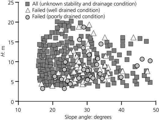
Selected 301 geometry combinations (74 failed slopes and 227 slopes of unknown stability) in cut slopes in medium- to high-plasticity clays from the NR earthwork portfolio (sources: Abbott, 2018; NR, 2017; Spink, 2020)
Selected 301 geometry combinations (74 failed slopes and 227 slopes of unknown stability) in cut slopes in medium- to high-plasticity clays from the NR earthwork portfolio (sources: Abbott, 2018; NR, 2017; Spink, 2020)
Material strength properties for medium- and high-plasticity clays forming the cut slopes within the NR data set
| Soil type | Peak | Fully softened or weathered | Residual | |||
|---|---|---|---|---|---|---|
| φ′: ° | c′: kPa | φ′: ° | c′: kPa | φ′: ° | c′: kPa | |
| London Clay | 22–28 | 23 | 20 | 12–16 | 14–15 | 0 |
| Oxford Clay | 22 | 0.5 | 21 | <0.1 | 16–11.5 | 0 |
| Lias Clays | 56 | 13–40 | 24 | <12 | 18–17 | 0 |
| Gault Clay | 33–53 | 47–124 | — | — | 12–15 | 0 |
| Atherfield Clay | 35 | — | 24 | 34 | 16–13 | 0 |
| Weald Clay | — | — | 24–22 | 10 | 16–15 | 0 |
Note: strength properties are shown for soils at the peak, fully softened and residual strength states (James, 1970)
Within the NR data set, there were 74 geometry combinations corresponding to recorded slope failures. Both the slope geometry and pore water pressure condition were known for these earthworks. This allowed the influence of pore water pressure conditions on slope failure to be considered for these particular cases. Failures recorded with a poorly drained condition consisted of slopes with heights ranging between 3 and 18 m and with angles of inclination between 12 and 61°. Failures recorded with a well-drained condition consisted of slopes with heights ranging between 3 and 19 m and with angles of inclination between 16 and 47°. In addition, NR records showed historical interventions (i.e. remediation) of slopes with heights ranging between 12 and 20 m and with angles of inclination between 21 and 63° (Spink, 2020).
Methodology
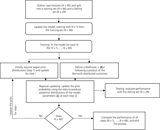
A Bayesian logistic model was used to classify the slope stability condition as a binary, dependent variable (stable or unstable). The section headed ‘Logistic regression for slope stability assessment’ describes the use of logistic regression for slope stability assessment, while the section headed ‘Bayesian logistic regression model and Bayesian updating’ describes the process of Bayesian logistic regression and the Bayesian updating approach. A summary of the modelling process, the Bayesian updating approach and the validation of the Bayesian updating approach is shown in Figure 2. It is worth noting that for the model, performing Bayesian updating on subsets of the training data is equivalent to standard Bayesian inference using the entire training data in the likelihood. In other words, the target posterior distribution using standard Bayesian inference is equivalent to the posterior distribution at the final step of the updating scheme in Figure 2 with N = 66. Here, Bayesian updating was performed on the training data to show how uncertainty decreases as more (live) data become available.
Logistic regression for slope stability assessment
Given that y (the overall condition of the slope) is a binary response, 1 for failure and 0 for stability, and x 1, x 2, x 3, x 4, x 5 and x 6 are continuous predictors (slope height, slope angle etc.), then the model can be used to predict the probability that a slope with specific characteristics corresponds to condition 1 (i.e. failure). A general model response is defined by Ohlmacher and Davis (2003):
where z i is the probability that a slope with specific characteristics failed and β = (β 0, …, β k) is the parameter’s vector of the unknown regression coefficients where k = 6 for the continuous predictors. The log odds can be transformed into the probability of the outcomes p i = p(y i = 1|x 1, x 2, …, x k) as follows:
Then, the probability of a slope corresponding to a failed or unstable condition is given by
where the slope height is H; the slope angle is α; the effective cohesion is c′; the effective friction angle is φ′; the unit weight is γ; and the pore water pressure coefficient is r u.
Bayesian logistic regression model and Bayesian updating
In a frequentist approach (i.e. the logistic regression described in the section headed ‘Logistic regression for slope stability assessment’), the parameters β j are considered fixed and unknown (i.e. single values or point estimates), and the only information used for inference are the data or observations. However, in a Bayesian approach, the parameters β j are random variables. This properly accounts for the uncertainty in the true parameter values (Bartolucci and Scrucca, 2010). The Bayesian approach combines expert knowledge with data observations for a particular phenomenon or parameter of interest to produce ‘posterior’ estimates using Bayes’s theorem. Expert knowledge about a parameter or process of interest is summarised by an appropriate probability distribution, also known as the prior distribution, whereas the probabilistic evidence provided by the observations is summarised by the likelihood (Richard, 2017), defined as L(β|y) in Figure 2. Hence, in a Bayesian logistic regression model, inference is used to find the posterior distribution of the unknowns. Bayes’s theorem states that the posterior distribution of a model parameter – for example, β j – is proportional to the product of the likelihood of observing the data given β j and its prior density. Therefore, the posterior beliefs around the Bayesian logistic regression coefficients are formed by both prior beliefs and the observed evidence (i.e. the data) (Contreras and Brown 2019).
Vague normal prior distributions were chosen for the regression coefficients, β j ∼ N(0, 10). The priors were then updated using the observed data according to a Bayesian updating scheme (Kyburg, 1987; Van de Schoot et al., 2021), a schematic diagram of which is shown in Figure 2. Bayesian updating is a stochastic method suited to geotechnical processes, particularly in the presence of limited information (Kelly and Huang, 2015). Bayesian updating is used to update the prior probability with new information, to then create a posterior probability. In this process, priors can be assumed based on experience or measured (or both) and are later reviewed. As new information about β j becomes available (i.e. considering more data from the whole set), the estimates are revised by updating the likelihood and estimating the posterior distribution to use as the new prior. In this study, an exercise was undertaken to demonstrate the effect that Bayesian updating and the availability of the new data had on the predictive accuracy of the model. The data set with N observations (70% of the available case histories, the training set with N = 66) was randomly divided to simulate a condition in which the initial available data were scarce, and subsequent updates were performed as data became available (N increased from N = 5 to N = 20 and then the complete training set, N = 66). As y i follows a Bernoulli distribution, the likelihood was obtained using a product of Bernoulli-distributed outcomes. This results in y i ∼ Bernoulli (p i) for p i corresponding to the outcome probability described by Equation 3, and the corresponding likelihood function is defined as , y = (y 1, …, y m)T. As the posterior distributions of β j are not analytically tractable, they were estimated using a Markov chain Monte Carlo (MCMC) procedure. By integrating the MCMC algorithm, posterior distributions were updated from prior distributions (Fattahi and Ilghani, 2020; Kass et al., 1998). Markov chains are stochastic models describing sequences of events, whereby each outcome determines the next outcome to occur according to a fixed set of probabilities. The chains are memoryless so that each event depends only on the one preceding it and does not include historical information (Geyer, 1992). The Bayesian analyses presented in this study were implemented in the Python programming language (Van Rossum and Drake, 2009) using the no-U-turn sampler. The latter is an MCMC algorithm that resembles Hamiltonian Monte Carlo but eliminates the need for choosing the number-of-steps parameter, making it an adaptively setting path length in Hamiltonian Monte Carlo (Hoffman and Gelman, 2014).
Model performance measurement
Once the posterior distributions of the model parameters were estimated, a testing set comprising 30% of the case histories (N = 29) was used to measure the predictive performance of the Bayesian model against unseen data (Figure 2). The performance was measured by assessing the occurrence of false positives and false negatives. The probability that an observation belongs to a condition y i was transformed into a binary response. If p i > 0.5, the observation was assigned to slope failure/instability (i.e. positive), and negative otherwise. Hence, true negatives were cases of stable slopes classified as stable and true positives were cases of unstable (or failed) slopes classified as unstable.
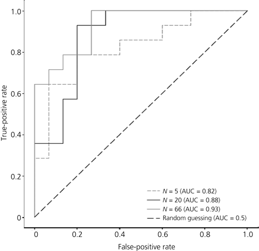
A receiver operating characteristic (ROC) curve was constructed, and the area under the curve (AUC) was determined. The ROC curve is a graphical plot that illustrates the diagnostic ability of a binary classifier system when the discrimination threshold is varied (Ai et al., 2010; Flach, 2016). The ROC was created by plotting the true-positive rate against the false-positive rate. The AUC measures the true-positive rate and false-positive rate trade-off, testing the quality of the value generated by a classifier (model) and then comparing the value to a threshold. The closer a curve is to the point (0, 1), the more accurate a predictor is. According to D’Agostino et al. (2018), AUC values above 0.85 show a high classification accuracy, values between 0.75 and 0.85 show a moderate accuracy and values less than 0.75 show a low accuracy. The AUC of the ROC showed the ability of the model to distinguish between conditions (in this study, the condition of a stable or unstable slope).
Evaluating clay cut slopes in the NR data set
The validated model, trained using the case history data, was used to determine the probability of failure for selected earthwork geometries within the NR data set. The slope geometric properties (slope height and angle) within the NR data set were known, but the pore water pressure condition and material properties were not always known. It is often not practical or affordable to measure slope strength properties across an earthwork asset portfolio, so this can be a source of uncertainty or omission within geotechnical asset data sets (Spink, 2020). Expert opinion and scenario testing have been used to structure problems and manage uncertainty within environmental models (Krueger et al., 2012; Uusitalo et al., 2015) and models of energy futures (Copeland et al., 2022). Scenarios were therefore used to define soil material property scenarios for the NR data set (Figure 3(a)). The choice of soil material property scenarios was informed by (a) published strength parameters for medium- and high-plasticity clay strata for UK cut slopes (Table 2) and (b) the time-dependent strength reduction of these medium- and high-plasticity clays due to the process of softening (Castellanos, 2013; Eid and Rabie, 2016; James, 1970; Mesri and Shahien, 2003; Stark and Eid, 1997; Trinidad Gonzalez et al., 2021b).
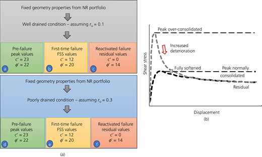
(a) Six material property and drainage condition scenarios for peak, fully softened and residual shear strength and for well-drained and poorly drained pore water pressure conditions; (b) shear characteristics of normally consolidated (black line) and over-consolidated (grey line) clays as defined by Skempton (1970). FSS, fully softened state
(a) Six material property and drainage condition scenarios for peak, fully softened and residual shear strength and for well-drained and poorly drained pore water pressure conditions; (b) shear characteristics of normally consolidated (black line) and over-consolidated (grey line) clays as defined by Skempton (1970). FSS, fully softened state
The strength scenarios included the transition from peak strength to the fully softened state (FSS) and residual strength with increasing strain and slope displacement (Figure 3(b)). This was observed in back-analyses of first-time slope failures in stiff, fissured clays that are typical of those in the NR data set (Skempton, 1964, 1970, 1977; Skempton and Petley, 1967). The scenarios represent pre-failure, first-time failure and reactivated failure conditions of the earthwork assets. The strength properties for London Clay in Table 2 were obtained from a greater number of laboratory tests and slope back-analyses than for the other strata and were therefore considered to be the more reliable and representative properties for the material condition. Therefore, the cut slopes within the NR data set were assigned material properties for three scenarios in London Clay. These were the material properties of London Clay at the peak, FSS and residual strength (Table 2). Similarly, the pore water pressure condition for many of the cut slopes within the NR data set was unknown. Therefore, the cut slopes were considered scenarios of either (a) a well-drained condition (r u = 0.1) or (b) a poorly drained condition (r u = 0.3), as shown in Figure 3.
The posterior distributions of the model parameters were obtained for each of the six scenarios, and the probability of failure was determined for each slope geometry in the NR data set using Equation 1. For example, for each model input x i in Equation 1, a value was given to the slope height, angle of inclination and unit weight. The pore water pressure coefficient, friction angle and cohesion values were selected for each of the six scenarios. The values of the posteriors for each model parameter (the coefficients of a Bayesian model) are shown in Figure 4. Equation 2 was used to transform the outcomes into probability distributions for the probability of slope failure. The mean of the probability distribution was used as a point estimate.
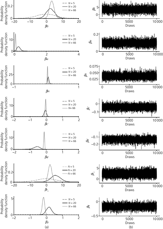
Posterior density plots (a) and trace plots (b) of the model parameters (at the training stage) for N = 5 and 20 and N = training set (70% of the case history data set, 66)
Posterior density plots (a) and trace plots (b) of the model parameters (at the training stage) for N = 5 and 20 and N = training set (70% of the case history data set, 66)
First, the mean probability of failure of the 74 failed cut slopes within the NR data set was determined for the three strength scenarios of peak, fully softened and residual shear strength, for each pore water pressure condition (a total of six scenarios; Figure 3). The mean probability of failure for the six scenarios and the known (failed) slope condition were used to identify the most probable material property and pore water condition scenarios for these failed slopes.
Finally, the Bayesian model was used to assess the probability of failure for the 227 slope geometry combinations with an unknown stability condition in the NR data set (Figure 1). An analysis was undertaken to determine the Bayesian model output sensitivity to each of the six inputs, for the range of values considered in the NR data set. The sensitivity analysis was conducted for the whole NR data set and the three material strength scenarios.
Results
Bayesian logistic regression model parameter inference
Figure 4 shows the posterior distribution of the Bayesian model parameters that were developed using the training set of published case histories. The results showed the density and trace plots of the posterior distributions and refinement of the credible intervals for the number of samples in the training set. The trace plot (shown in Figure 4) of the MCMC sample draws (β j against time) was examined to identify anomalies and evaluate convergence. For most of the parameters, the posterior variance was significantly reduced when compared with the prior distribution variance, particularly as the available information increased and the prior distributions were updated at each step (Figure 2).
Model performance
The ROC and the respective AUC of the model, evaluated with the testing set, are shown in Figure 5. The latter shows that the predictive performance of the model improved as the N increased from N = 5 to N = 20 and N = 66. Figure 5 also shows that models with N > 20 were able to predict stable or unstable slopes with a high classification accuracy (AUC > 0.85).
Probability of failure for clay cut slopes in the NR data set
Figure 6 shows the mean probability of failure for geometries corresponding to the 74 failed slopes (45 well-drained slopes and 29 poorly drained slopes) within the NR data set. Results are shown for the three material strength scenarios (peak, fully softened and residual strength) for the well-drained and poorly drained conditions. Figure 6 shows that peak strength scenarios (scenarios (a) and (d)) are less likely than the scenarios for deteriorated soil strength. For slope failures with a poorly drained pore water pressure condition, the highest probabilities of failure correspond to the residual strength scenario (f). The model predicted a probability of failure of at least 60% for most of these poorly drained, residual strength slopes. For the same drainage condition, the results showed a higher probability of failure for short, steep slopes in the fully softened strength scenario (e) than for well-drained slopes. For slope failures with a well-drained pore water pressure condition, the results showed the highest probability of failure for the residual strength condition (scenario (c)), followed by the fully softened strength condition (scenario (b)). This showed that the recorded failures in both well-drained and poorly drained NR cut slopes were more likely to have mobilised a reduced shear strength relative to the peak condition. Failures in short (<10 m) and less steep (<35°) slopes could be the result of repeated failures and reparations that caused the residual strength to be mobilised. This agreed with the observations of reactivated failures in many NR earthworks (Spink, 2020).
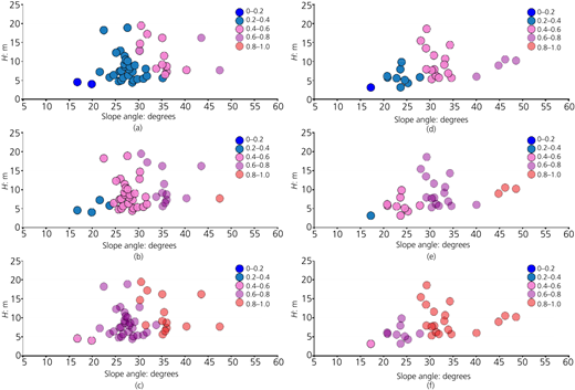
Probability of failure for 74 failed slopes recorded in the NR data set, for well-drained and poorly drained scenarios and strength transition from peak strength to the FSS and residual strength: (a) peak strength well-drained; (b) FSS strength well-drained; (c) residual strength well-drained; (d) peak strength poorly drained; (e) FSS strength poorly drained; (f) residual strength poorly drained
Probability of failure for 74 failed slopes recorded in the NR data set, for well-drained and poorly drained scenarios and strength transition from peak strength to the FSS and residual strength: (a) peak strength well-drained; (b) FSS strength well-drained; (c) residual strength well-drained; (d) peak strength poorly drained; (e) FSS strength poorly drained; (f) residual strength poorly drained
Figure 7 shows the mean probability of failure for the 227 unique slope angle and height combinations in the NR data set for the most critical scenarios ((b), (c), (e) and (f)) from Figure 6. The results show that steeper slopes (>35°) have higher probability of failure than shallower slopes, irrespective of slope height. The results of the Bayesian model show that if the mobilised strength of an NR cut slope is at the fully softened strength, and a well-drained pore water pressure condition is maintained (a), slopes steeper than 25° have at least a 40% probability of failure, irrespective of their height. However, if the drainage condition of these slopes falls to the poorly drained state for the same strength condition (b), the same probability of failure (>40%) applies to all slopes steeper than 19° (i.e. a greater proportion of slopes).
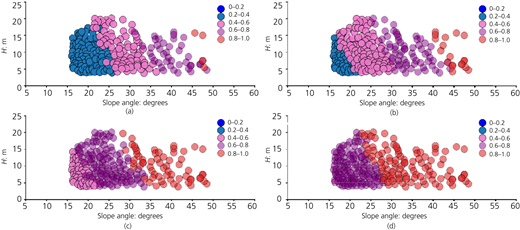
Probability of failure for 227 geometry combinations within the NR cut slope data set with soil strength at the fully softened (FSS) and residual conditions for well-drained and poorly drained pore water pressure conditions: (a) FSS strength well-drained; (b) FSS strength poorly drained; (c) residual strength well-drained; (d) residual strength poorly drained
Probability of failure for 227 geometry combinations within the NR cut slope data set with soil strength at the fully softened (FSS) and residual conditions for well-drained and poorly drained pore water pressure conditions: (a) FSS strength well-drained; (b) FSS strength poorly drained; (c) residual strength well-drained; (d) residual strength poorly drained
The results from Figure 7 show that if the soil strength is at the residual state, irrespective of the drainage condition ((c) and (d)), the probability of failure is at least 40%. The probability significantly increases to at least 60% when transitioning from a well-drained to a poorly drained pore water pressure condition (scenario (d)). A comparison of the results based on strength conditions (a) and (b) against (c) and (d) shows a significant increase in the probability of failure for the scenario of a mobilised shear strength at the residual state. Part (a) in Figure 7 shows that slopes with H > 10 m and an angle of inclination of 25° have a 20% higher probability of failure than shorter slopes with the same angle of inclination. However, once the drainage and strength conditions become less favourable, the effect of the slope height on the probability of failure is reduced (as shown in (b)–(d)). Figure 7 shows that the pore water pressure condition considerably influences the probability of failure for a given slope geometry. Therefore, an understanding of the slope drainage condition is a priority for the assessment of cut slope stability. It is worth noting that the results shown in Figures 6 and 7 are a representation of an idealised scenario where the material properties of all assets are represented by an average soil, and the whole soil mass is assumed to mobilise uniform values of strength. It can therefore be used to identify the characteristics of earthwork slopes with the highest probability of failure and to inform risk-based prioritisation programmes for tactical asset management and further investigation. However, the assessment of individual slopes at the operational level would require more traditional investigation and analysis approaches, incorporating site-specific factors, to assess their stability.
The results from the sensitivity analysis are shown for each strength condition (Figure 8(a)), and all scenarios (Figure 8(b)) in terms of log-worth. The log-worth is a p-value transformation also known as the S-value, based on the Pearson chi-squared test (Greenland, 2019; Good, 1956; Rafi and Greenland, 2020; Shannon, 1948). The log-worth values shown are −log transformations of the p-value of each model effect. The higher the log-worth, the higher the model effect. Figures 8(a) and 8(b) show that the slope angle of inclination has the greatest contribution to the variability of the mean probability of slope failure. These results are in agreement with the findings presented by Svalova et al. (2021) whereby a surrogate model was created to evaluate the time to failure (TTF) for earthwork slopes using experimental design and FD analyses. Svalova et al. (2021) concluded that the slope angle cotangent had the greatest contribution to the variability of the slope stability response. The Svalova et al. (2021) geometry combinations with an angle cotangent below 2 (≈26°) showed the shortest TTF (TTF ≤ 50 years). This is in agreement with the results shown in Figure 7 for most drainage conditions. This shows that steeper slopes in the NR data set have the highest likelihood of failure. Figures 8(a) and 8(b) show that the second most influential factor is the pore water pressure coefficient, which represents the drainage condition. The slope geometry has a reduced influence on the probability of slope failure as the strength decreases from the peak to the residual condition (Figure 8(a)), representing the pre-failure and reactivated failure scenarios.
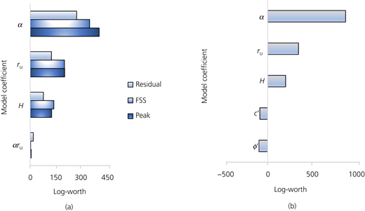
Sensitivity analysis of the effects of input properties on the probability of failure considering 227 geometries within the NR data set for (a) the three strength scenarios considered separately and (b) all scenarios considered together
Sensitivity analysis of the effects of input properties on the probability of failure considering 227 geometries within the NR data set for (a) the three strength scenarios considered separately and (b) all scenarios considered together
The results from Figures 7 and 8 can be used to rank the slopes and identify the earthworks with the highest likelihood of slope failure. For example, if the acceptable threshold for probability of failure is p > 40% , for slopes in materials prone to softening with no record of past failures ((a) and (b) in Figure 7), the results indicate that the assets in a well-drained condition will be stable. This will result in a probability of failure below the 40% threshold for slopes with an angle of inclination less than 25°. However, slopes with H > 10 m will require a well-drained condition to satisfy the threshold. Under the same conditions, slopes with an angle of inclination greater than 25° require a well-drained condition to satisfy the threshold, irrespective of their height. In the presence of records of any previous failure and repair and a well-maintained well drainage condition ((c) in Figure 7), slopes with an angle of inclination as low as 20°, irrespective of their height, require a well-drained condition to satisfy the acceptable threshold.
Conclusions
A Bayesian logistic regression model combining published case histories and a Bayesian updating approach was used to predict the likelihood of failure of ageing clay slopes within an earthwork asset portfolio. A Bayesian approach was considered in preference to traditional deterministic, mechanical modelling analyses (i.e. LE analyses) in order to consider a large number of slope geometries for different material and drainage conditions. However, the Bayesian approach was limited to six predictors and was therefore not able to consider all the site-specific information about individual slopes. For a more detailed assessment of individual slopes, a traditional physical modelling analysis would be more appropriate. A Bayesian approach was preferred to other soft computing techniques because of its ability to deal with limited or missing data and extract causal relationships from relatively small data sets. This makes it particularly suited to the examination of earthwork asset portfolios such as the one examined in this paper. As more information about the NR assets becomes available, or if the method is applied to an asset portfolio with more detailed information, the model can be updated to improve the predictions.
The following can be concluded from the use of a Bayesian updating approach to consider the stability of railway earthwork slopes.
The probability of failure was determined from knowledge of the slope geometry, soil properties and the pore water pressure condition. The model was able to predict the slope stability condition (stable or unstable) with a high classification accuracy using a training data set of published slope failure case histories. This was shown by the AUC of the ROC > 0.85. The results showed that the performance of the Bayesian model increased with each Bayesian updating step.
The Bayesian model was used to rank the probability of failure of 227 medium- and high-plasticity clay cut slopes within an NR data set, based on the measured slope geometry and on scenarios of material properties and pore water pressure conditions. This compared well with recorded failures in the NR data set. The rank probability showed that the scenarios of residual strength compared most closely with the failure records in the NR data set. This reflected the age of these assets, where many slope failures could be first-time or reactivated failures, with degraded material strength at the residual state.
The sensitivity analyses showed that the probability of failure increased with the slope angle, for slopes with peak material strength at the pre-failure state. However, the probability of failure was less sensitive to the slope angle for slopes with fully softened or residual material strength, representing first-time failures and reactivated failures, respectively. The second most influential factor was the slope pore water pressure condition, particularly for shallower slopes (<35°) at deteriorated states of fully softened to residual shear strength. Therefore, steep slopes (well-drained and poorly drained) had the highest probability of failure within an asset portfolio of ageing cut slopes at deteriorated soil strength states, such as those in the NR data set. However, for less steep slopes (<35°), poorly drained slopes had an approximately 20% higher probability of failure than well-drained slopes. These findings can inform the risk-based prioritisation of slopes within the NR data set for further investigation.
The material properties for the failed cut slopes in the NR data set were unknown. Therefore, the uncertainty was managed using scenarios for slope material properties based on published laboratory tests and slope back-analyses. However, as specific information becomes available for individual stable and failed slopes within the NR data set, the Bayesian model can be updated to improve the probability estimates and alter the failure threshold values. The probability distribution function from the Bayesian model can also be used for probabilistic assessments of slope stability, rather than the deterministic results presented in this study.
Acknowledgements
This work was supported by the Engineering and Physical Sciences Research Council-funded Achilles Programme (EP/R034575/1), with thanks to the industrial advisory panel including Network Rail and chaired by Dr Chris Power of Mott MacDonald. Kevin Briggs is supported by the Royal Academy of Engineering and HS2 Ltd under the Senior Research Fellowship scheme (RCSRF1920\10\65).
Appendix
A case history data set was used to train and validate the Bayesian model for a range of slope geometries and material types. The data set (Table 3) included information from 95 case histories, consisting of 41 stable slopes and 54 unstable slopes that had failed due to a rotational failure mechanism.
Details of the 95 slope stability case histories summarised by Trinidad González et al. (2021a) from Manouchehrian et al. (2014) and Sah et al. (1994), showing the slope height (H), the slope angle (α), the pore water pressure coefficient (r u), the effective friction angle (φ′), the effective cohesion (c′), the unit weight (γ) of the soil and the slope stability condition
| Case study | H: m | α: ° | c′: kPa | φ: ° | r u | γ: kN/m3 | Stability condition |
|---|---|---|---|---|---|---|---|
| 1 | 8.23 | 35 | 26 | 15 | 0.00 | 18.68 | Failed |
| 2 | 3.66 | 30 | 11 | 0 | 0.00 | 16.50 | Failed |
| 3 | 30.50 | 20 | 14 | 25 | 0.00 | 18.84 | Stable |
| 4 | 100.00 | 35 | 29 | 35 | 0.00 | 28.44 | Stable |
| 5 | 100.00 | 35 | 39 | 38 | 0.00 | 28.44 | Stable |
| 6 | 40.00 | 30 | 16 | 27 | 0.00 | 20.60 | Failed |
| 7 | 50.00 | 20 | 0 | 17 | 0.00 | 14.80 | Failed |
| 8 | 88.00 | 30 | 12 | 26 | 0.00 | 14.00 | Failed |
| 9 | 6.00 | 30 | 25 | 0 | 0.00 | 18.50 | Failed |
| 10 | 6.00 | 30 | 12 | 0 | 0.00 | 18.50 | Failed |
| 11 | 10.00 | 30 | 10 | 35 | 0.00 | 22.40 | Stable |
| 12 | 20.00 | 30 | 10 | 30 | 0.00 | 21.40 | Stable |
| 13 | 50.00 | 45 | 20 | 36 | 0.00 | 22.00 | Failed |
| 14 | 50.00 | 45 | 0 | 36 | 0.00 | 22.00 | Failed |
| 15 | 4.00 | 35 | 0 | 30 | 0.00 | 12.00 | Stable |
| 16 | 8.00 | 45 | 0 | 30 | 0.00 | 12.00 | Failed |
| 17 | 4.00 | 35 | 0 | 30 | 0.00 | 12.00 | Stable |
| 18 | 8.00 | 45 | 0 | 30 | 0.00 | 12.00 | Failed |
| 19 | 10.67 | 22 | 25 | 13 | 0.35 | 20.41 | Stable |
| 20 | 12.19 | 22 | 12 | 20 | 0.41 | 19.63 | Failed |
| 21 | 12.80 | 28 | 9 | 32 | 0.49 | 21.82 | Failed |
| 22 | 45.72 | 16 | 34 | 11 | 0.20 | 20.41 | Failed |
| 23 | 10.67 | 25 | 15 | 30 | 0.38 | 18.84 | Stable |
| 24 | 7.62 | 20 | 0 | 20 | 0.45 | 18.84 | Failed |
| 25 | 61.00 | 20 | 0 | 20 | 0.50 | 21.43 | Failed |
| 26 | 21.00 | 35 | 12 | 28 | 0.11 | 19.06 | Failed |
| 27 | 30.50 | 20 | 14 | 25 | 0.45 | 18.84 | Failed |
| 28 | 76.81 | 31 | 7 | 30 | 0.38 | 21.51 | Failed |
| 29 | 88.00 | 30 | 12 | 26 | 0.45 | 14.00 | Failed |
| 30 | 20.00 | 45 | 24 | 30 | 0.12 | 18.00 | Failed |
| 31 | 100.00 | 20 | 0 | 20 | 0.30 | 23.00 | Failed |
| 32 | 10.00 | 45 | 10 | 35 | 0.40 | 22.40 | Failed |
| 33 | 50.00 | 45 | 20 | 36 | 0.25 | 20.00 | Failed |
| 34 | 50.00 | 45 | 20 | 36 | 0.50 | 20.00 | Failed |
| 35 | 50.00 | 45 | 0 | 36 | 0.25 | 20.00 | Failed |
| 36 | 50.00 | 45 | 0 | 36 | 0.50 | 20.00 | Failed |
| 37 | 8.00 | 33 | 0 | 40 | 0.35 | 22.00 | Stable |
| 38 | 8.00 | 33 | 0 | 40 | 0.30 | 24.00 | Stable |
| 39 | 8.00 | 20 | 0 | 25 | 0.35 | 20.00 | Stable |
| 40 | 8.00 | 20 | 5 | 30 | 0.30 | 18.00 | Stable |
| 41 | 90.50 | 50 | 17 | 28 | 0.25 | 27.30 | Stable |
| 42 | 92.00 | 50 | 26 | 31 | 0.25 | 27.30 | Stable |
| 43 | 6.00 | 30 | 25 | 0 | 0.25 | 18.50 | Failed |
| 44 | 6.00 | 30 | 12 | 0 | 0.25 | 18.50 | Failed |
| 45 | 10.00 | 30 | 10 | 35 | 0.25 | 22.40 | Stable |
| 46 | 20.00 | 30 | 10 | 30 | 0.25 | 21.40 | Stable |
| 47 | 50.00 | 45 | 0 | 36 | 0.25 | 22.00 | Stable |
| 48 | 4.00 | 45 | 0 | 30 | 0.25 | 12.00 | Stable |
| 49 | 8.00 | 45 | 0 | 30 | 0.25 | 12.00 | Failed |
| 50 | 4.00 | 45 | 0 | 30 | 0.25 | 12.00 | Stable |
| 51 | 8.20 | 35 | 9 | 15 | 0.00 | 18.66 | Failed |
| 52 | 100.00 | 35 | 10 | 35 | 0.00 | 28.40 | Stable |
| 53 | 6.00 | 30 | 8 | 0 | 0.00 | 18.46 | Failed |
| 54 | 20.00 | 30 | 3 | 30 | 0.00 | 21.36 | Stable |
| 55 | 10.60 | 22 | 8 | 13 | 0.35 | 20.39 | Stable |
| 56 | 12.20 | 22 | 4 | 20 | 0.41 | 19.60 | Failed |
| 57 | 45.80 | 16 | 11 | 11 | 0.20 | 20.39 | Failed |
| 58 | 21.00 | 35 | 4 | 28 | 0.11 | 19.03 | Failed |
| 59 | 8.00 | 20 | 2 | 30 | 0.30 | 17.98 | Stable |
| 60 | 12.00 | 40 | 7 | 40 | 0.00 | 20.96 | Stable |
| 61 | 12.00 | 40 | 12 | 28 | 0.50 | 20.96 | Stable |
| 62 | 6.00 | 34 | 3 | 29 | 0.30 | 19.97 | Stable |
| 63 | 50.00 | 25 | 10 | 10 | 0.10 | 18.77 | Stable |
| 64 | 50.00 | 30 | 10 | 20 | 0.10 | 18.77 | Stable |
| 65 | 50.00 | 30 | 8 | 20 | 0.20 | 18.77 | Failed |
| 66 | 40.00 | 30 | 5 | 27 | 0.00 | 20.56 | Failed |
| 67 | 3.60 | 30 | 4 | 0 | 0.00 | 16.47 | Failed |
| 68 | 30.60 | 20 | 5 | 25 | 0.00 | 18.80 | Stable |
| 69 | 30.60 | 20 | 19 | 20 | 0.00 | 18.80 | Stable |
| 70 | 100.00 | 35 | 13 | 38 | 0.00 | 28.40 | Stable |
| 71 | 6.00 | 30 | 4 | 0 | 0.00 | 18.46 | Failed |
| 72 | 10.00 | 30 | 3 | 35 | 0.00 | 22.38 | Stable |
| 73 | 50.00 | 45 | 7 | 36 | 0.00 | 21.98 | Failed |
| 74 | 10.60 | 25 | 5 | 30 | 0.38 | 18.80 | Stable |
| 75 | 30.60 | 20 | 5 | 25 | 0.45 | 18.80 | Failed |
| 76 | 76.80 | 31 | 2 | 30 | 0.38 | 21.47 | Failed |
| 77 | 88.00 | 30 | 4 | 26 | 0.45 | 13.97 | Failed |
| 78 | 20.00 | 45 | 8 | 30 | 0.12 | 17.98 | Failed |
| 79 | 15.00 | 45 | 33 | 45 | 0.25 | 22.38 | Stable |
| 80 | 10.00 | 45 | 3 | 35 | 0.40 | 22.38 | Failed |
| 81 | 50.00 | 45 | 7 | 36 | 0.25 | 19.97 | Failed |
| 82 | 50.00 | 45 | 7 | 36 | 0.50 | 19.97 | Failed |
| 83 | 12.00 | 49 | 15 | 25 | 0.30 | 20.96 | Stable |
| 84 | 12.00 | 40 | 10 | 35 | 0.40 | 20.96 | Stable |
| 85 | 15.00 | 30 | 13 | 30 | 0.30 | 19.97 | Stable |
| 86 | 14.00 | 25 | 15 | 25 | 0.30 | 17.98 | Stable |
| 87 | 11.00 | 35 | 10 | 35 | 0.20 | 18.97 | Stable |
| 88 | 10.00 | 40 | 13 | 40 | 0.20 | 19.97 | Stable |
| 89 | 37.00 | 29 | 8 | 21 | 0.50 | 18.83 | Failed |
| 90 | 37.00 | 34 | 3 | 21 | 0.30 | 18.83 | Failed |
| 91 | 50.00 | 25 | 8 | 10 | 0.20 | 18.77 | Failed |
| 92 | 50.00 | 25 | 7 | 10 | 0.30 | 18.77 | Failed |
| 93 | 50.00 | 25 | 3 | 10 | 0.40 | 19.08 | Failed |
| 94 | 50.00 | 30 | 7 | 20 | 0.30 | 18.77 | Failed |
| 95 | 50.00 | 30 | 3 | 20 | 0.40 | 19.08 | Failed |
