
A significant portion of railway network income is spent on the maintenance and restoration of the railway infrastructure to ensure that the networks continue to provide the expected level of service. The execution of the interventions – that is, when and where to perform maintenance or restoration activities, depends on how the state of the infrastructure assets changes over time. Such information helps ensure that appropriate interventions are selected to reduce the deterioration speed and to maximise the effect of the expenditure on monitoring, maintenance, repair and renewal of the assets. Presently, there is an explosion of effort in the investigation and use of data-driven methods to estimate deterioration curves. However, real-world time history data normally includes measurement of errors and discrepancies that should not be neglected. These errors include missing information, discrepancies in input data and changes in the condition rating scheme. This paper provides solutions for addressing these issues using machine learning algorithms, estimates the deterioration curves for railway supporting structures using Markov models and discusses the results.
Notation
Introduction
As infrastructure continuously deteriorates, stakeholders must be able to predict its deterioration speed to determine the optimal maintenance programs. Although there are different types of models used for this purpose (Setunge and Hasan, 2011), Markov and semi-Markov models, have perhaps been the most extensively used ones for management purposes (Kobayashi et al., 2012; Nam, 2009). For example, Madanat et al. (1995), Robelin and Madanat (2007) and Setunge and Hasan (2011) used Markov models to predict bridge deterioration curves and Ortiz-Garcia et al. (2006) used them to model the pavement deterioration. Manafpour et al. (2018) used a semi-Markov time-based model to model concrete bridge deck deterioration, and Edirisinghe et al. (2015) predicted the building deterioration using a Markov model.
In general, the Markov models use data from inspections of the condition state (CS) of the infrastructure over time to estimate the deterioration curves. Consequently, the quality of data plays a significant role in the accuracy of deterioration prediction and the resulting lifecycle cost estimations. Recently, there has been significant progress towards more frequent and accurate monitoring of the assets and storage of the related results. However, real-world data often do not exist in sufficient quantity, contain errors and discrepancies and are not always suitable for estimating the transition probabilities. These issues and errors often result from failure to achieve the results of past inspections (lack of history), missing information or faulty entries, lack of a robust guideline for condition assessment, the discrepancies between the judgment of inspectors and the measurement of errors related to machines, equipment, sensors and so on.
Researchers have also done work to bridge these gaps for Markov models. Specifically, Mizutani et al. (2017) suggested improving the estimation of Markov transition probabilities using mechanistic-empirical models, and Lethanh et al. (2017) used these models along with Monte Carlo simulations to estimate the transition probabilities for a reinforced concrete bridge element with chloride-induced corrosion. Humplick (1992) has studied methods to tackle the issues of measurement errors related to monitoring equipment and measurement locations. Park et al. (2008) and Hong and Prozzi (2006) have used a Bayesian approach to deal with the small population samples for pavement deterioration prediction. Chu and Durango-Cohen (2007, 2008) used Kalman filters to eliminate errors in pressure and deflection measurements for asphalt pavements and provided numerical examples to demonstrate how their framework accommodated the missing values. So far, researchers have mostly addressed issues related to the equipment, location or measurement errors related to humans such as faulty entries and discrepancies in the judgements of the inspectors (Kobayashi et al., 2012). There are occasions, however, where there is a systematic discrepancy among the data entries, such as changes in the condition rating system, that have not been addressed in the literature.
This paper contributes to the literature by examining a real-world case study to predict the deterioration curves of the railway supporting structures using Markov models. In this study, state-of-the-art tools were used to clean the data and deal with the faulty or incomplete entries. Moreover, three classification algorithms – that is, K-nearest neighbours (KNNs), neural networks (NNs) and random forest algorithms were used to adjust a portion of the data collected using an old condition rating scheme to the equivalents with a new condition rating scheme.
Study description
This paper developed the deterioration curves for railway supporting structures from a data set with faulty or incomplete entries, inaccuracies related to the inconsistent monitoring programs and biased data, as well as to the situation where there were changes in the CS rating system. The supporting structures in this study were bridges and retaining walls that laterally support soil to restrain it at different levels on the two sides.
An inventory of the assets containing 4988 bridges and 17 000 retaining walls were created in the years 1983 and 2000, respectively, and the results of regular inspections were entered in a database following that date. In the asset inventory, each object was assigned a unique identification number, and the document provided information on the type of construction and materials, the dimensions, the position of the object, the construction year and the results of the inspections. The bridges were classified into four categories: masonry, steel, concrete and composite. The retaining walls were divided into three categories according to their structural behaviour – that is, gravity, cantilever and anchored walls, and further three categories according to their primary construction material, namely, masonry, concrete and natural stone.
Material-wise, they were divided into three categories: masonry, concrete and natural stone walls. For all structures, the inspections were performed every six years on average, which resulted in a total of 26 106 status reports from 1983 to December 2018 for bridges, and 52 647 status reports from the year 2000 to February 2020 for the retaining walls. These status reports indicated the CS of the objects at the time of inspection. The CSs ranged between 1 and 5, where 1 represents the best state and 5 represents the worst. These conditions are basically attributed based on the presence of visible damage to the structure and the resulting intervention costs or traffic hindrances. Hence, the assigned states are very descriptive and prone to subjectivity. The first change in the condition rating scheme occurred in 2009 and affected all objects. The second change occurred in 2013 and affected only natural stone-retaining walls (see Figure 1).
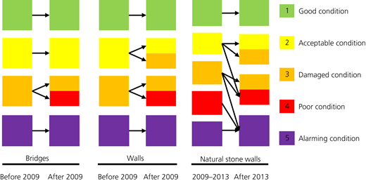
Changes in the condition-rating scheme of all objects in 2009 and the natural stone retaining walls in 2013
Changes in the condition-rating scheme of all objects in 2009 and the natural stone retaining walls in 2013
The following steps were used to develop the deterioration curves:
data cleaning and preparation
estimation of the transition probabilities using Markov models
approximation of the deterioration curves and the dwell times – that is, the duration that the structures stay in each CS, using the transition probabilities and Monte Carlo simulations.
The following sections discuss these steps more in detail.
Data preparation
Data cleaning
In the first step, the set of data was cleaned and structured for use in the estimation of the transition probabilities. The faulty or incomplete entries were first corrected or deleted if unusable, but with the aim of keeping as many entries as possible to have the most informative value for the models.
Two main assumptions were made in dealing with missing data. Objects with missing inspection data, where the former and later inspection campaigns showed the same CS, were considered to have maintained this CS the whole time. For example, if an object was supposed to be inspected every five-to-six years but there was a 12-year gap between two available inspection data, both assigning a CS2 to the object, it was assumed that the object had been in CS2 the whole time.
The second assumption was when an object at time t was in CS X and then, after 12 years, was degraded one level CS (X + 1). In such situations, it was assumed that the CS changed to X + 1 only at t = 12 and not before.
Dealing with changing rating schemes
In the second step, the problem of the variations in the condition rating scheme was addressed. Four CSs were used prior to 2009 for all object types and five CSs afterwards. Also, the classification criteria for natural stone walls became stricter in 2013, meaning that worse CSs were assigned to objects after 2013 than before. Hence, CSs before and after 2009 and 2013 could not be directly compared (Figure 1).
This problem was addressed by reclassifying the inspection results (CSs) that happened before the changes in the rating system. The basic idea for the reclassification was to estimate the CSs using other information available in the database, such as wall type and material, construction year and damage type. As this could be done in different ways, the performance of three classification algorithms, KNN, NN and the random forest, were compared together to adjust the past CSs to the currently used CSs. The CSs of the natural stone-retaining walls before 2009 were first adjusted for the first rating change and then again for the second rating change in 2013. Brief overviews of the classification methods used in this study with their related advantages and limitations are provided in the Appendix.
As can be seen in Figure 1, for bridge inspections before 2009, bridges with the CS1 and CS2 maintained the same CS, those with CS3 could either be CS3 or CS4, and bridges with a CS4 would be classified as CS5. For the retaining wall inspections before 2009, walls with the CS CS1 maintained the same CS, those with CS2 could either be CS2 or CS3, walls with CS3 could be either CS3 or CS4, and walls with a CS4 would be classified as CS5. Additionally, for stone walls, CSs reported before 2013 were treated as follows: (a) walls with CS1 were still considered as CS1; (b) walls with the CS2 could be either CS2, CS3 or CS4; (c) walls with CS3 could be in CS3, CS4 or CS5; and (d) walls with CS4 and CS5 were considered to be in CS5. This meant that a total of five reclassifications were required.
1) Reclassify the old CS3 (all bridges before 2009).
2) Reclassify the old CS2 (all walls before 2009).
3) Reclassify the old CS3 (all walls before 2009).
4) Reclassify the old CS2 (natural stone walls before 2013).
5) Reclassify the old CS3 (natural stone walls before 2013).
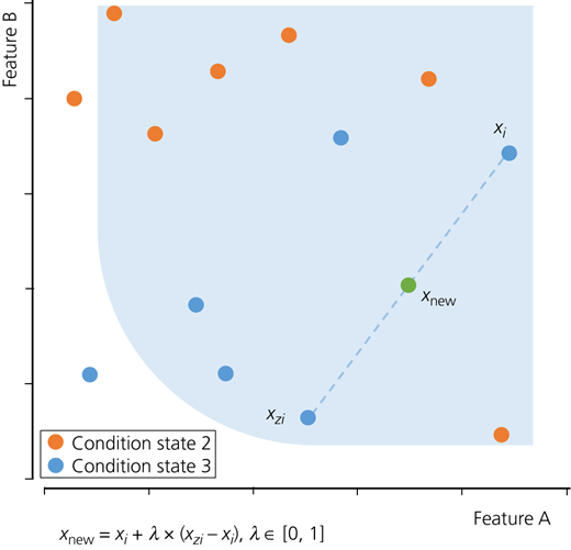
After an initial assessment of the number of observations for each CS, it was observed that the distribution of data entries for each CS, for both bridges and walls, was very skewed and unbalanced. For example, the data record for the retaining walls contained 12 394 status entries of CS2 and 2979 status entries of CS3. When dealing with an unbalanced dataset such as this one, the classification algorithms predict the CS too optimistically, since there are many more entries in CS2 than in CS3. This is because the frequency of entries in each CS is learned in the training dataset, such that the skewed distribution is reflected in the predicted CSs. To ensure that the classification only takes place based on the informative value of the features and not on the relative frequency of occurrence of the individual CSs, the training dataset was modified (augmented) to have the same number of entries for each CS.
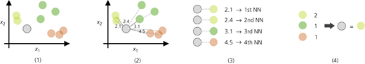
Two methods of data augmentation, namely, oversampling and synthetic minority oversampling technique (SMOTE), were used to deal with the problem of the skewed dataset. In oversampling, copies of the features of the minority class(es) were created until the number of entries in the minority class(es) were the same as the class with the highest number of data entries. SMOTE synthesised new entries for the minority class(es) rather than duplicating them. This algorithm uses the concept of the KNN and selects data points in the minority class that are close to the feature space, draws a line between the data points and adds a new entry at a point along that line. Figure 2 provides an insight as to how the new data entry is generated.
For each of the algorithms, two-thirds of the data points were used as the training set and one-third as the evaluation set, and the features (input values) were normalised. The choice of features was tailored according to each classification algorithm – that is, with the random forest and the NN, all available features (related to the damage type, material, wall type, the year of construction and the distance to the track axis) were used; as these classification algorithms used a weighing scheme for the features and as sufficient data points were available, their performance was not negatively affected when all features were used. With the KNN algorithm, a feature selection algorithm was first applied to only consider the most meaningful features. The reason was that the KNN algorithm can achieve higher accuracy when there were fewer features involved. In general, to reduce the number of features, either a principal component analysis (PCA) or a ‘feature selection’ procedure is carried out (Witten et al., 2011). In this study, a ‘backward elimination’ technique (Kittler, 1978; Marill and Green, 1963) for feature selection was used and the most significant features (i.e. the construction year, material and damage mechanism) were selected to be used in the KNN classifier. These features were those that correlated most strongly with the CSs. For bridges, features based on the material (masonry, steel, concrete, composite), features based on the damage type (corrosion, damage to the cover, damage to the support structure) and the construction year had the highest correlations with the CSs. For retaining walls, features based on the material (natural stone and reinforced concrete), features based on wall categories (gravity walls, cantilever walls and anchored walls), features based on the damage type (damage to the cover and damage to the support structure) and the construction year had the highest correlations with the CSs.
In the next step, a so-called ‘parameter tuning’ was carried out for all classification algorithms, and the combination of parameters that resulted in the best performance was selected for each algorithm. The performance of the algorithms can be compared using various measures. For example, ‘accuracy’ is the most common performance measure that represents the ratio of correctly predicted observations to the total observations. The f 1 score is another measure that is not as easy to understand as accuracy but is more useful, especially when dealing with uneven class distributions. For this reason, we used the f 1 score for comparing the algorithms. This score is calculated as
where in a classification problem with two classes of positive and negative, precision is the ratio of the true-positive observations to the total predicted positive observations; and recall is the ratio of the true-positive observations to the sum of true-positive and false-negative observations (i.e. all observations in actual positive class). The results of the best combinations of parameters for each algorithm are summarised in Table 1.
Selected parameters for KNN, NN, and random forest algorithms
| Algorithm | The selected combination of parameters | Comments |
|---|---|---|
| KNN | k =15 | The number of closest neighbors for classification 1, 2 and 3 |
| k =20 | The number of closest neighbors for classification 4 and 5 | |
| NN | n_hidden = 3 | The number of hidden layers |
| h_size = (50, 50, 50) | Hidden layer size | |
| φ = tanh | Activation function [logistic, tahn, relu] | |
| α = 0.01 | Learning rate | |
| Random forest | max_depth = 100 | The maximum depth of the tree |
| max_features = sqrt | The number of features to consider when searching for a suitable split | |
| min_samples_split = 2 | The minimum number of samples required to split an internal node | |
| n_estimators = 100 | The number of trees in the forest |
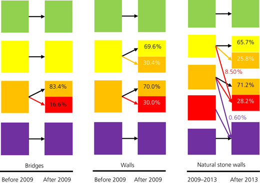
Table 2 summarises the performance of the algorithms (f 1 scores) on the evaluation set for each algorithm with original data (normal) and the data augmented with oversampling and SMOTE. It can be observed from Table 2 that the random forest algorithm delivered better classification results, followed by the NN and the KNN algorithm. Also, data augmented with oversampling led to better performance of the classifiers in comparison to SMOTE and the original training set (normal). Figure 3 provides the results of the four classification tasks. The percentages on the arrows show the proportion of the data with the old rating scheme that is transferred to a new CS. For example, for retaining walls, for the inspections that were carried out before 2009, 69.6% of the CS2 states maintained the same CS, while 30.4% were demoted to CS3 according to the new condition rating scheme.
Performance of the KNN, NN and random forest algorithms
| Classification algorithm | KNN | NN | Random forest | |||||||
|---|---|---|---|---|---|---|---|---|---|---|
| Aggregation of the training data set | Normal | Oversampled | SMOTE | Normal | Oversampled | SMOTE | Normal | Oversampled | SMOTE | |
| Classification 1 | f 2 score | 0.569 | 0.547 | 0.584 | 0.587 | 0.603 | 0.612 | 0.723 | 0.763 | 0.745 |
| Classification 2 | f 2 score | 0.538 | 0.592 | 0.592 | 0.564 | 0.614 | 0.591 | 0.714 | 0.749 | 0.730 |
| Classification 3 | f 2 score | 0.530 | 0.566 | 0.565 | 0.680 | 0.684 | 0.650 | 0.809 | 0.811 | 0.800 |
| Classification 4 | f 2 score | 0.401 | 0.456 | 0.444 | 0.473 | 0.460 | 0.434 | 0.682 | 0.699 | 0.695 |
| Classification 5 | f 2 score | 0.377 | 0.429 | 0.335 | 0.551 | 0.632 | 0.572 | 0.793 | 0.862 | 0.795 |
In the next step, the data were further refined and structured for the development of the deterioration curves for each category of bridges and retaining walls.
Data structuring
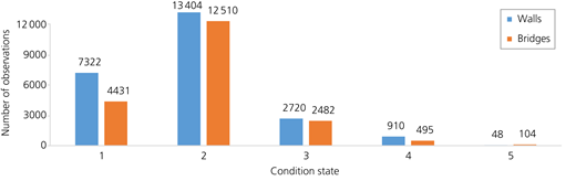
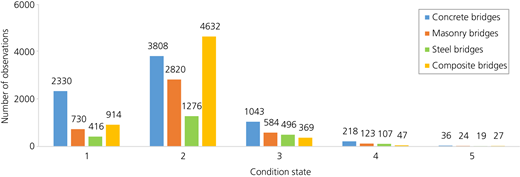
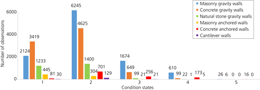
Figure 4 illustrates the recorded CSs of the bridges and retaining walls after the data cleaning and preparation. The x-axis shows the CS of the objects, and the y-axis shows the number of observations (each data point represents an inspection result). After data preparation, a total of 20 022 (out of 26 106) status entries for bridges and 24 479 (out of 52 647) status entries for retaining walls remained. This shows that the retaining walls had lost more than half of their observations due to duplicated or incomplete entries in the retaining wall data inventory. Moreover, most of the observations belong to the first three CSs and only 3.15 and 0.3% of them belong to CS4 and CS5, respectively.
The bridges and walls were then divided into suitable categories to develop more accurate and informative data-based decay curves. The aim was to group the objects based on the distinct features that could significantly influence their deterioration rate while keeping the number of groups as small as possible to ensure sufficient data points per category. Figures 5 and 6 show the categories of bridges and retaining walls respectively along with the number of observations per CS for each category of objects.
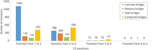
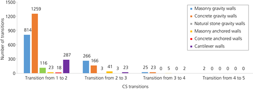
In the next step, a sequence of the CS transitions was created to develop the transition probabilities for each bridge and retaining wall based on the results of the inspections. These sequences could not contain improvements in the CS. However, if all objects that were ever repaired were filtered out, too many data points would be lost. To avoid this issue, the sequences of CS transitions were adjusted as follows:
If there was an improvement in the CS of an object and this observation was confirmed twice in succession, it was assumed that the object was renewed. Consequently, the sequence was divided into two separate ones as if the second sequence belonged to a newly constructed object. For example, the wall i with CS sequence CS i = {1,1,2,3,1,1,2}, was split into two sequences CS i = {1,1,2,3} and CS i +1 = {1,1,2}.
In a sequence, where the improvement in the CS only happened once and then returned to a worse state, such as in CS i = {1,2,1,2,3}, the improvement was considered as an inconsistency in the judgment of the inspectors and hence, it was corrected as CS i = {1,2,2,2,3}.
A further issue with the current dataset was related to the lack of history, as the database only contained the results of inspections from the year 1983 to 2018 for bridges and 2000 to 2020 for the retaining walls. This denotes that information on the condition development of the objects before this period was missing. For example, a retaining wall was built in 1970 but was only added to the database in 2006 with a CS1. In 2010, a degradation to CS2 was reported. However, it is unknown whether between 1970 and 2006, the wall stayed in CS1 or underwent one or more condition improvement interventions. Hence, there is a lower bound of 4, and an upper bound of 40 years for the dwell time in CS1, depending on the condition history of this wall. Since assuming that no interventions were executed before the first inspection would result in optimistic and non-conservative results, the period between the year of construction and the initial inspection was not taken into account. This approach, although conservative, allowed for keeping the entries without the construction year as the data analysis could be carried out using Markov models. Figures 7 and 8 illustrate the recorded CS transitions for each category of bridges and walls.
Transition probabilities
Markov models were used to estimate the deterioration curves. Markov models are stochastic processes that provide predictions of the future development of a process with limited knowledge of its history (see the paper of Parzen (1962) and the book of Howard (1971) for more detailed information). Hence, they were very suitable for modelling the deterioration curves of the railway supporting structures (i.e. bridges and retaining walls), as the information on the development of the CSs was only available from the initial inspection of the objects and not from the year of construction.
The bridge and wall deterioration transition probability matrices would be upper triangular (Equation 2) since, in a natural deterioration process, there cannot be improvements in the CSs (without interventions). Moreover, CS5 would be the absorbing state, as there was no way to get out of this state without taking repairing measures.
A regression-based optimisation was used to estimate the transition probabilities (Roelfstra et al., 2004). The objective function of this approach (Equation 3) was to minimise the sum of the absolute differences between the CS at time, t, based on the regression curve, C(t), and the expected CS at time, t, based on the Markov chain and the estimated probabilities, E(t) (Bulusu and Sinha, 1997).
where N is the total number of the transition periods and S is the CS vector. For the bridges and retaining walls, the expected CS at time t – that is, E(t) can be expressed as
Assuming xtj denotes the proportion of objects in CSj at time interval t, the objective function of the optimisation problem in Equation 3 can be written as
The matrix x(t − 1) has a dimension of [(t − 1) * j; j2], the vector of the transition probabilities, pij, has a dimension of [j2; 1] since i = j and the vector x(t) has a dimension of [(t − 1) * j; 1].
The process of estimating the transition probabilities starts with data aggregation within a certain time interval, Δt. For the bridges since the age of the objects were known, the Δt was selected as 5 over a period of 100 years (20 time intervals), and then the proportion of the number of observations in each CS was calculated in each time interval, considering the age of the bridge. For the walls, as the information regarding the year of construction was unknown for almost half of the walls, the time of the first inspection for all walls was considered as t0 and only the time differences between the inspections were considered. As the inspections in the database were conducted from the year 2000 to 2020, 20 time intervals (Δt = 1) were selected for data aggregation to estimate the transition probabilities for each category of retaining walls.
In this problem, t ∈ {1,2,3,…,20} denotes the interval number and i, j ∈ {1,2,3,4,5} represent the CSs. Subsequently, the transition probabilities were estimated using the regression-based approach described above. The optimal solutions to Equation 6 – that is, the transition probability matrices for each category of the bridges and retaining walls are presented in Tables 3 and 4. It can be observed that due to the lack of sufficient observations in CS5, CS4 was the absorbing state for all wall categories except masonry gravity walls. Moreover, the number of observations in CS4 and CS3 were much lower than CS2 and CS1, which suggests that these CSs trigger intervention activities from the management authorities to avoid dangerous CSs.
Deterioration curves and dwell times
After data preparation and estimation of the transition probabilities, a fictitious portfolio of 12 000 objects was created for each category of bridges and retaining walls. The deterioration of the objects over time was then simulated using the estimated transition probabilities and the Monte Carlo simulations. The dwell times for each CS were then calculated based on the results of the previous step (Figures 9 and 10). Tables 5 and 6 provide a comparison between the dwell times of bridges and retaining walls derived directly from the data (i.e. the max, min and the mean time that each category of bridges and retaining walls was in each CS based on the inspection data) and the estimated dwell times using the developed transition probabilities and the Monte Carlo simulations.
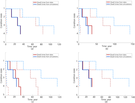
Estimated dwell times for each category of bridges: (a) concrete bridges; (b) masonry bridges; (c) steel bridges; (d) composite bridges. Solid lines indicate the mean dwell time, while the dashed lines (--) show the minimum, and the dotted dashed lines (-·-) show the maximum values
Estimated dwell times for each category of bridges: (a) concrete bridges; (b) masonry bridges; (c) steel bridges; (d) composite bridges. Solid lines indicate the mean dwell time, while the dashed lines (--) show the minimum, and the dotted dashed lines (-·-) show the maximum values
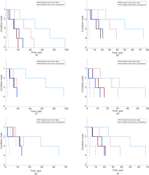
Estimated dwell times for each category of walls: (a) masonry gravity walls; (b) concrete gravity walls; (c) natural stone walls; (d) masonry anchored walls; (e) concrete anchored walls; (f) cantilever walls. Solid lines indicate the mean dwell time, while the dashed lines (--) show the minimum values, and the dotted dashed lines (-·-) show the maximum values
Estimated dwell times for each category of walls: (a) masonry gravity walls; (b) concrete gravity walls; (c) natural stone walls; (d) masonry anchored walls; (e) concrete anchored walls; (f) cantilever walls. Solid lines indicate the mean dwell time, while the dashed lines (--) show the minimum values, and the dotted dashed lines (-·-) show the maximum values
Estimated dwell times for bridges
| Concrete bridges | |||||||
|---|---|---|---|---|---|---|---|
| Type | Condition state | μ | σ | Median | Min | Max | Observations |
| Dwell times from data | 1 | 12.86 | 6.58 | 11.71 | 0.00 | 31.97 | 1330 |
| 2 | 13.48 | 8.61 | 11.58 | 0.08 | 35.20 | 388 | |
| 3 | 6.94 | 3.89 | 5.81 | 1.94 | 16.11 | 15 | |
| Dwell times from simulations | 1 | 13.39 | 9.94 | 11.00 | 1.00 | 38.00 | 10 547 |
| 2 | 13.35 | 8.88 | 12.00 | 1.00 | 37.00 | 3997 | |
| 3 | 6.09 | 5.04 | 4.00 | 1.00 | 33.00 | 2844 | |
| Masonry bridges | |||||||
| Type | Condition state | μ | σ | Median | Min | Max | Observations |
| Dwell times from data | 1 | 10.30 | 4.76 | 10.93 | 0.00 | 32.23 | 176 |
| 2 | 13.62 | 7.96 | 11.59 | 0.00 | 34.96 | 284 | |
| 3 | 12.69 | 5.14 | 12.70 | 4.46 | 20.86 | 16 | |
| Dwell times from simulations | 1 | 8.89 | 8.01 | 6.00 | 1.00 | 50.00 | 11 968 |
| 2 | 10.98 | 9.21 | 8.00 | 1.00 | 48.00 | 7812 | |
| 3 | 6.40 | 5.70 | 5.00 | 1.00 | 44.00 | 11 178 | |
| Steel bridges | |||||||
| Type | Condition state | μ | σ | Median | Min | Max | Observations |
| Dwell times from data | 1 | 10.50 | 5.24 | 10.17 | 0.84 | 25.47 | 116 |
| 2 | 12.17 | 6.67 | 11.59 | 0.33 | 30.04 | 141 | |
| 3 | 6.80 | 3.04 | 5.95 | 0.92 | 12.29 | 23 | |
| 4 | 4.62 | 0.00 | 4.62 | 4.62 | 4.62 | 1 | |
| Dwell times from simulations | 1 | 5.22 | 4.65 | 4.00 | 1.00 | 40.00 | 11 997 |
| 2 | 11.93 | 9.02 | 10.00 | 1.00 | 39.00 | 10 682 | |
| 3 | 7.46 | 6.16 | 6.00 | 1.00 | 36.00 | 9124 | |
| Composite bridges | |||||||
| Type | Condition state | μ | σ | Median | Min | Max | Observations |
| Dwell times from data | 1 | 11.26 | 5.46 | 11.03 | 0.00 | 27.95 | 422 |
| 2 | 15.83 | 8.15 | 15.84 | 0.00 | 32.65 | 506 | |
| 3 | 7.96 | 4.24 | 5.98 | 0.23 | 21.57 | 57 | |
| Dwell times from simulations | 1 | 10.22 | 9.00 | 7.00 | 1.00 | 45.00 | 11 851 |
| 2 | 16.15 | 10.92 | 14.00 | 1.00 | 44.00 | 6505 | |
| 3 | 6.65 | 5.57 | 5.00 | 1.00 | 41.00 | 5297 | |
Estimated dwell times for retaining walls
| Masonry gravity walls | |||||||
|---|---|---|---|---|---|---|---|
| Type | Condition state | μ | σ | Median | Min | Max | Observations |
| Dwell times from data | 1 | 6.27 | 2.64 | 5.87 | 0.00 | 14.17 | 814 |
| 2 | 6.32 | 2.54 | 5.92 | 0.01 | 15.36 | 266 | |
| 3 | 4.94 | 2.81 | 5.40 | 0.04 | 11.86 | 25 | |
| 4 | 2.59 | 2.58 | 2.59 | 0.00 | 5.17 | 2 | |
| Dwell times from simulations | 1 | 3.56 | 2.93 | 3.00 | 1.00 | 23.00 | 3944 |
| 2 | 10.30 | 6.73 | 9.00 | 1.00 | 25.00 | 6190 | |
| 3 | 7.88 | 5.75 | 7.00 | 1.00 | 25.00 | 4347 | |
| 4 | 6.35 | 4.92 | 5.00 | 1.00 | 25.00 | 2887 | |
| Concrete gravity wall | |||||||
| Type | Condition state | μ | σ | Median | Min | Max | Observations |
| Dwell times from data | 1 | 6.32 | 2.36 | 5.96 | 0.00 | 14.58 | 1259 |
| 2 | 5.92 | 2.14 | 5.84 | 0.08 | 15.38 | 166 | |
| 3 | 5.74 | 2.14 | 5.94 | 0.22 | 9.11 | 23 | |
| Dwell times from simulations | 1 | 4.54 | 3.87 | 3.00 | 1.00 | 25.00 | 6277 |
| 2 | 11.26 | 6.84 | 11.00 | 1.00 | 25.00 | 2966 | |
| 3 | 5.18 | 4.33 | 4.00 | 1.00 | 25.00 | 3655 | |
| Natural stone gravity walls | |||||||
| Type | Condition state | μ | σ | Median | Min | Max | Observations |
| Dwell times from data | 1 | 6.49 | 2.27 | 5.93 | 0.26 | 11.87 | 116 |
| 2 | 5.84 | 0.24 | 5.67 | 5.67 | 6.17 | 3 | |
| Dwell times from simulations | 1 | 5.71 | 5.04 | 4.00 | 1.00 | 33.00 | 9887 |
| 2 | 8.30 | 6.69 | 6.00 | 1.00 | 33.00 | 11 185 | |
| 3 | 4.33 | 3.65 | 3.00 | 1.00 | 30.00 | 10 717 | |
| Masonry anchored walls | |||||||
| Type | Condition state | μ | σ | Median | Min | Max | Observations |
| Dwell times from data | 1 | 5.50 | 2.26 | 5.87 | 1.79 | 13.21 | 23 |
| 2 | 5.90 | 2.09 | 5.90 | 0.93 | 11.44 | 41 | |
| 3 | 5.74 | 0.68 | 6.01 | 4.39 | 6.14 | 5 | |
| Dwell times from simulations | 1 | 1.44 | 0.76 | 1.00 | 1.00 | 6.00 | 856 |
| 2 | 6.80 | 5.53 | 5.00 | 1.00 | 26.00 | 8223 | |
| 3 | 4.74 | 3.94 | 4.00 | 1.00 | 26.00 | 10 378 | |
| Concrete anchored walls | |||||||
| Type | Condition state | μ | σ | Median | Min | Max | Observations |
| Dwell times from data | 1 | 5.85 | 1.21 | 5.81 | 3.44 | 8.20 | 18 |
| 2 | 5.85 | 0.66 | 6.07 | 4.95 | 6.53 | 3 | |
| Dwell times from simulations | 1 | 1.41 | 0.75 | 1.00 | 1.00 | 7.00 | 2710 |
| 2 | 9.69 | 6.17 | 9.00 | 1.00 | 22.00 | 5136 | |
| 3 | 2.13 | 1.52 | 2.00 | 1.00 | 15.00 | 6332 | |
| Cantilever retaining walls | |||||||
| Type | Condition state | μ | σ | Median | Min | Max | Observations |
| Dwell times from data | 1 | 6.57 | 2.56 | 5.93 | 0.87 | 14.26 | 287 |
| 2 | 5.96 | 1.89 | 5.58 | 3.11 | 12.68 | 23 | |
| 3 | 8.74 | 2.87 | 8.74 | 5.87 | 11.61 | 2 | |
| Dwell times from simulations | 1 | 6.04 | 5.08 | 4.00 | 1.00 | 25.00 | 5615 |
| 2 | 11.30 | 6.83 | 11.00 | 1.00 | 25.00 | 1833 | |
| 3 | 2.68 | 2.17 | 2.00 | 1.00 | 18.00 | 3478 | |
The comparison between the dwell times derived directly from inspection data and the dwell times estimated using transition probabilities and Monte Carlo simulations shows that the wall and bridge categories with a higher number of observations produced more accurate estimations of the transition probabilities. This can vividly be seen through the comparison of the dwell times for concrete and composite bridges, where the estimated dwell times are almost equal to the dwell times from inspection data (Figure 9). In these categories, although the minimum and mean dwell times are almost the same, the max dwell times from the simulations are considerably longer. Here, it seems that the simulations likely provide a better reflection of reality than the data because the max dwell times from the data are constrained due to the limited period of time over which the data were collected. For example, in Table 5, the maximum dwell time derived from data for concrete bridges in CS2 is 35.2, which is equal to the max inspection history. In contrast, the Monte Carlo simulations show a longer maximum dwell time because for a ‘fictitious’ bridge, the dwell time is not constrained.
For the masonry bridges and steel bridges, there were discrepancies among the dwell times derived from data and those estimated using the simulations. This was mainly due to the lack of sufficient observations in these categories (Table 5). For the retaining walls (Table 6 and Figure 10), the discrepancies were more noticeable. For example, for all wall categories, the dwell times estimated for CS2 using the simulations were higher than those observed directly from data due to overestimation of the transition probability, p22. This was principally due to the fact that the number of CS2 observations is higher than the rest of the CSs, and secondly, due to the accumulation of aggregated observations in the first few time intervals, which occurred because the year of construction was unknown for almost half of the retaining walls. To deal with this issue as mentioned in Section 3.3, when preparing the data, the initial inspections for all walls were set to t = 0, while this was not the case in reality as the walls were of different ages, and the first inspections were not actually carried out at the same time. This approach was selected as it allowed for keeping the entries without the construction year and also had the advantage of being ‘representative’ for all available time intervals (Δt = 1), whereas for the bridges where the chronological order of the first inspections in time was used (i.e. not set to be at t = 0), a ‘representative deterioration time interval’ was selected to estimate the transition probabilities (Δt = 5) which was also consistent with the use of Markov models.
In general, it may be noticeable that the dwell times might seem to many experts as relatively short. The predominant reason for this was most likely due to the significance of the CSs on the object level and their use in practice. Although the CSs are expected to demonstrate how the object is deteriorating over time in practice, the assigned CSs are associated with the worst state of an element, which alert management to the fact that an intervention is required in the near future, even if it is small. Hence, the sum of the dwell times in each CS for an asset does not correspond with the total amount of time that it is expected to be in service before it needs to be replaced. This difference is because in one particular case, CSs are used to approximate the life of the asset, and in the other, they are being used to trigger interventions.
Conclusions
Determination of optimal intervention programs for infrastructure depends on the development of the CS of the assets over time. Markov models are appropriate models that use the information from the CS development of the assets over time and predict their deterioration rate and the remaining service life. This paper used a Markov model to predict the deterioration curves of the railway bridges and retaining walls and proposed solutions to address the challenges that normally exist when dealing with real-world data, including insufficient inspection history, incomplete/faulty entries, biased data caused by the lack of clear guidelines for the inspectors and the changes to the condition rating scheme.
It is concluded that the following considerations can be made in other similar situations in practice:
The data should be cleaned by correcting or deleting the faulty or incomplete entries. This is done to preserve as many entries as possible to increase the informative value of the models.
While structuring the data, a distinction must be made between the situations where there are discrepancies between the judgment of inspectors and the situations where there have been improvements in the condition of the structures due to maintenance work.
The old inspection data must be adjusted in accordance with the new rating scheme when there is a change in the condition rating system. In this study, KNN, NN and random forest were used for reclassification purposes and to align the inspection data with the new condition rating schemes, so that the data obtained before and after the changes in the condition rating scheme could be compared with each other. The results suggested that the random forest was the most appropriate method for this classification problem.
The transition probability matrices can be estimated using a regression-based optimisation approach for each category of objects. The deterioration curves and dwell times can be estimated by using the transition probabilities in conjunction with Monte Carlo simulations.
When there is no information on the construction year of the objects in the database, in using the Markov models, the period between the year of construction and the initial inspection can be neglected and the initial inspections for all objects should be set to t = 0. This would result in the conservative estimation of the transition probabilities except for the CS that had the highest concentration of the observations in the first few intervals.
One simple but occasionally neglected way to mitigate data losses due to faulty entries in the repositories would be using a drop-down menu rather than the manual insertion of the information. Additionally, to avoid biases in the inspection ratings, the condition rating scheme should be revised to be strict and clear, leaving no room for interpretations.
To obtain more accurate estimates of the deterioration process with limited data, it is advisable to determine mechanistic-empirical deterioration models for each individual retaining wall category and then calibrate the results using the available data.
The application of automated structural health monitoring or drone-based surveillance systems can facilitate regular collection of data from all assets, for future developments of the deterioration curves.
The difference between the different uses of CSs has to be considered – that is, one cannot simply take the CSs reported in data and use them directly to estimate the expected lifetime of the asset.
Acknowledgements
The authors would like to thank the financial support of the Fonds de Recherche du Québec – Nature et Technologies (FRQNT) and the Natural Sciences and Engineering Research Council of Canada (NSERC).
Appendix
The K-nearest neighbour
The K-nearest-neighbour (KNN) algorithm is a simple, but very efficient classification method. The key idea behind the KNN classification is that similar measured values belong to the same classes. Thus, one only needs to know the class identifier of a certain number of the nearest neighbours to be able to estimate the class number of a data point (Figure 11). The class of an unknown data point is usually determined using the majority criterion – that is, if the majority of the neighbours of an unknown point are from class A, it is very likely that the point is also from class A.
The advantages of this method include the ease of implementation and not needing a training period. However, this algorithm does not work well with large data sets and high dimensions, needs feature scaling, and is sensitive to missing values, outliers, and noisy data. Also, in this method, the number of nearest neighbours k should be kept as small as possible since a large k can lead to a bad classification if the individual classes are not well separated.
Neural networks
NNs are computational models with the capacity to learn, generalise or classify data. NNs are beneficial in approximating unknown non-linear functions that depend on a large number of variables (features) since their application eliminates the need to define that function. Figure 12 represents a typical single-layer NN classifier. The model contains an input layer of variables (features), a hidden layer and an output layer with the desired classes In addition to the normal neurons, there are also bias neurons that are used to help ensure that the model has a good fit with existing data. The weights (connections between neurons) are used to model the relationships between the neurons. The activation function is used to introduce non-linearity into the model to ensure that there is a good fit between the values predicted by the model and the expected output. To use these models, the network needs to be trained first – that is, the weights are adjusted (by going through a certain number of forward and backward propagations) so that the error between the expected output and the generated output of the model is minimised.
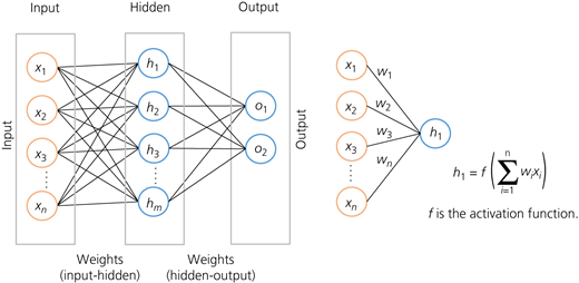
In a trained NN classifier, an input data point with known characteristics (features) is passed to the first hidden layer, where the activation function in each neuron receives the input xi and generates the output. That output is then passed to the next hidden layer (if any) and the procedure continues till it reaches the output layer, where outputs from the previous layer are combined to yield a final class of the input data point.
An NN can work with missing information, which makes it very suitable when dealing with an incomplete dataset. However, the algorithm requires training and there is no specific rule for determining the structure of the network and the task is done through experience or trial and error.
Random forest
Random forests are built from decision trees and are widely used for classification and regression problems. Fundamentally, they structure multiple hierarchical sequences of yes/no questions that ultimately lead to a decision. The variety of decision trees is what makes random forests more effective than individual decision trees. The random forest algorithm determines the class of an unknown data point using the following steps:
1. Create a bootstrapped dataset.
2. Create a decision tree using the bootstrapped dataset, only using a random subset of the variables (features) at each step.
3. Repeat steps 1 and 2, i times (i being the number of created decision trees or estimators).
4. Take the unclassified data and run it down on each decision tree, to find the class of the data point using various decision trees.
5. The class of an unknown data point is determined using the majority criterion – that is, the class that receives the most votes from the decision trees is chosen.
Similar to NN, random forest can handle missing information, is robust to outliers and less impacted by noisy data and is suitable for both classification and regression problems. Additionally, the algorithm reduces the variance and the overfitting problem in decision trees and improves the accuracy. However, it is computationally expensive as it develops a lot of trees and has a relatively long training period.
