Test selection in the twenty-first century

Article Type: Tutorial section From: Journal of Modelling in Management, Volume 7, Issue 3

This tutorial demonstrates how a regression-based analytical system can replace the more traditional cook-book approach that still commonly forms the basis of many introductory statistical courses in the social sciences. Analyses based on generalized linear models (GLMs) offer significant advantages in terms of their flexibility and power and also offer a much simpler system for teaching; one that is based on a solid theoretical base. The huge selection of hypothesis tests that are available may be represented using, essentially, a single model, which can be applied to different types of data and study design. Comparison analyses are provided in this tutorial to illustrate the superiority of a regression-based approach. It is proposed that regression models should replace the out-dated hypothesis-testing approach that for some reason still seems to dominate the social sciences.

It is very common in social science research to compare groups in order to ascertain whether statistically significant differences exist. For example,“do male and female employees have different perceptions about promotion prospects?”, “is educational level related to attitude?”,“has a certain intervention strategy affected production output?” and“is the socio-economic status of parents related to their children’s physical health?”. Selecting an appropriate statistic to test such hypotheses is a basic analytical skill, but is one that frequently causes problems, particularly for students who rely on “traditional” tests such as the t-test, ANOVA, Mann-Whitney, Kruskal-Wallis, Friedman and the χ² tests for contingency tables. There are a bewildering number of tests available and selection is often the result of using simple tables or flow-charts on the basis of decisions about the number of variables involved, the number of groups compared, the design of the study and the level of measurement of the dependent variable (see, for example, Motulsky,2010 and Motulsky, 2012 for examples of tables for selecting statistical tests). Although an appropriate test may be identified using these tables, this process of test selection is broadly a-theoretical and does not help students to understand the following questions:

• Why may a particular test be applied?

• What assumptions are/have been made?

• How can problems be tested and rectified?

• How can the test be generalized to accommodate different designs, different types of data or additional variables? Or even

• How should the data be structured to enable a statistical analysis to be carried out?

Many of these difficulties can, however, be addressed by the use of regression models. These allow statistical tests to be easily identified,detailed diagnostics to be applied, additional variables to be added and different research designs accommodated. The use of regression models is particularly relevant as many traditional tests are simply standard regression models that are restricted to certain conditions[1]. These restrictions were once necessary, since the tests were developed at a time when the complexity of arithmetical calculations needed for a more unified approach excelled the resources generally available. The widespread availability of microcomputers and statistical software, such as the R language (R Development Core Team, 2012),have changed this situation completely. Pencils, paper, books of log-tables and slide-rules have been replaced by efficient, easy to use statistical computing environments that have facilitated the migration from a plethora of special cases to an approach based on a single, logically-consistent structure.

Regression analyses not only provide identical results to the traditional parametric tests, they also provide a number of additional benefits. One of the major benefits of using GLMs is that the regression models have a consistent underlying theory that can be extended to model different types of data,including ordered and unordered categorical and count data. This enables the large range of tests available for parametric and non-parametric data to be replaced with a small number of GLMs that provides the user with a unified theory for test selection and also offers significant advantages with respect to the quality of analysis.

Put concisely, the continued propagation of “pen and paper techniques”represents a bounding factor for both the modern organization, be it educational or commercial, and for the individual, who chooses to remain in the statistical Stone Age. In their excellent introduction to statistical thinking, Diggle and Chetwynd (2011) summarize these thoughts very elegantly:

[…] restricting the statistical recipe book to explicit formulae is unnecessary. Far better […] to adopt a principled approach to statistical analysis, in which the old “which test can I use on my data?” mantra is replaced by “how can I use statistical thinking to help me get the best possible answer to my scientific question?”

A short comment on statistical models

Although the notion of a statistical model will be familiar to the reader on an intuitive level, the concept is used almost universally without even the most basic explanation. This tutorial advocates statistical modelling within the uniform, overarching framework of GLMs. It is therefore perhaps wise to outline the concept somewhat, not only to avoid misconceptions but also to motivate the reader to mull over statistical goals, rather than unconsciously using the“model” as just another unavoidable ingredient in the statistical soup.

It would also be all too easy to start an abstract mathematical discussion of statistical models, filling page after page with notation that may be logically satisfying, but probably bereft of any useful content for the task at hand. The interested reader is directed towards Dekking et al. (2005) for an excellent formal introduction to statistical thought, and to McCullagh (2002),which offers an exacting but interesting discussion of some aspects of statistical models.

Lindsey (1998) fixes the role of statistical modelling firmly within the context of the subject of study:

Any data collected contain a mass of information. The problem is for you to extract that part of it that is relevant to the questions to be answered by your study, in the simplest and most understandable way possible. This essentially involves checking for pertinent patterns and anomalies in the data. This is a basic role of statistical models: to simplify reality in a reasonable and useful way, a way that you can empirically check with the data.

“The formalization of variability, as an approximation to reality, is known as a statistical model” (Lindsey, 1995). This formalization of variability (on the sample space of interest) occurs through one or more(parametrized) statistical distributions, producing a mathematical abstraction of reality that captures the fundamental characteristics of interest.

The importance of the connection between the model and reality cannot be stressed too strongly. Concentrating on goodness of fit attributes between data and model, while condemning such thoughts as “does this really make sense?”to a subservient role may cause little real damage in academic circles, but when perpetrated in the real world may have grave consequences. We advocate the use of a consistent, understandable and flexible framework in order to free up practitioners so that they may concentrate on the subject matter, and not to ease the manufacture of sub-standard analyses:

If a particular model (parametrization) does not make biological sense, this is a reason to exclude it from the set of candidate models, particularly in the case where causation is of interest (Burnham and Anderson, 2002).

A regression-based approach

This section discusses how traditional tests can be mapped onto linear models. In its simplest form, the relationship between a dependent variable and an independent variable (also known as the response and explanatory variables)can be represented by the model:

The ~symbol signifies a link between the variables X and Y, and the form of this relationship depends on the distribution of the Y variable (McCullagh and Nelder, 1989). This model simply states that variable “Y” may be related to, i.e. dependent on, variable “X”. Examples of such relationships are:

• the score achieved in a mathematics test may be related to gender;

• the attitude of an employee may be related to their status within the company; and

• the likelihood of injury may be related to the wearing of safety equipment.

Y can be measured on any scale (see Stevens, 1946 for a discussion of measurement scales) and helps identify the specific technique used for the model. If, for example, Y is continuous, an ordinary least squares (OLS)regression model may be used; should Y be categorical, a logit regression model may be more appropriate, and if Y is a count or frequency variable, a Poisson regression may be used. With the application of appropriate dummy-variable coding techniques, variable X can also be measured on any scale (see Hutcheson,2011a, c, for a tutorial on dummy-variable coding).

When X is an unordered categorical variable (e.g. gender, group, or company),the model Y ~ X compares scores between the group categories for independent observations, i.e. different subjects provide scores for each category. This model is an independent-groups design and is represented using a regression model format as:

This model represents the traditional group tests for independent samples. For example, when Y is a continuous variable, the model is an OLS regression which is equivalent to an independent groups ANOVA (or a t-test, if there are just two group categories). If Y is ordered categorical, a proportional-odds logit model may be used. This replaces non-parametric tests such as the Mann-Whitney and Kruskal-Wallis. If Y is unordered categorical, a multinomial logit model may be used which is equivalent to a χ²contingency table analysis (contingency table cell-counts can also be analysed using a Poisson regression model that directly models count data[2]). Many of these analyses and the “equivalent” traditional tests are demonstrated below.

The regression models are particularly versatile as additional information available to the analyst can be accounted for by adding extra variables into the model. For example, if the samples from the study are drawn from different schools or companies, this information may be simply added into the model:

Extending the simple model Y ~ X, the above states that variable “Y” may be related to, i.e. dependent on, variables “group” and “company”. The regression model is, essentially, the same as before and a regression technique based on the measurement of Y is applied. It is not easy, however, to adapt the traditional tests to account for additional variables, as this changes the test that may be applied.

The ability to add additional variables has an added benefit in that it makes it easy to account for different research designs. For example, matched-groups designs can be analysed by simply adding the information about matching. For example, in a repeated measures design, a single subject is represented in more than one group category (for example, when individual subjects rate a number of different stores). A regression model for a matched-groups design simply includes both the “group” and “subject” variables:

The additional information about subject is added to the model as an unordered categorical variable. This model represents the traditional group tests for dependent samples. For example, when Y is a continuous variable, the model is an OLS regression, which is equivalent to an dependent groups ANOVA (or a paired t-test, if there are just two group categories). If Y is ordered categorical, a proportional-odds logit model may be used, which replaces the non-parametric tests such as’the Wilcoxon and Friedman. If Y is unordered categorical, a multinomial logit model may be used which is equivalent to a multi-way contingency table analysis.

The important thing to note here is that all of the traditional group group tests can be analysed using the GLM “Y ~ group” and an appropriate dummy coding scheme[3]. In addition to providing a simpler structure for group tests, the regression models provide a number of other advantages. The ability to add additional variables to the model enables more complex hypotheses to be tested (these models reproduce or replace the two-way ANOVAs, ANCOVAs and the equivalent non-parametric tests). This is particularly important given the non-experimental nature of many research studies[4]. The regression models also allow easy access to diagnostic tools and data transformations.

These models may appear simplistic, but they reproduce or replace the traditional hypothesis tests and provide a much simpler and more powerful system of analysis. Table I shows a list of traditional tests[5] (ordered according to the number of independent variables and the research design) and the corresponding, i.e. replacement, regression models.

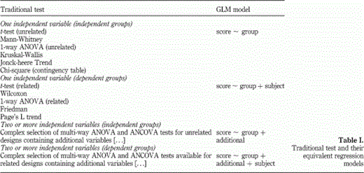
Table I Traditional test and their equivalent regression models

Demonstrating the analyses

It is useful to demonstrate that the traditional parametric tests can be reproduced and that the non-parametric tests may be replaced with regression models. Table II shows an example dataset which contains minimal data required to run the analyses. It should be noted that analyses are just for demonstration and are not intended to be accurate models (the dataset is far too small to represent the population). All statistics have been computed in R (R Development Core Team, 2012) with analysis of deviance tables reported for all regression models (see Fox and Weisberg, 2011 and Hutcheson and Moutinho, 2008, for discussions of deviance in regression).

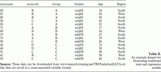
Table II An example dataset for illustrating traditional tests and regression models

A. Reproducing traditional parametric tests using regression

Traditional tests for parametric data (for example, t-tests, ANOVA,ANCOVA) are special cases of regression and can be reproduced using OLS regression models. The following examples show the same analyses conducted on 2 and 3 category groups on data collected from independent and dependent group studies.

Independent groups

A one-way ANOVA or an OLS regression model may be used to test whether there is a difference in “score.num” (a continuous variable) between the groups (indicated by variable “group”) for data collected using an independent-groups design.

Traditional test: one way ANOVA

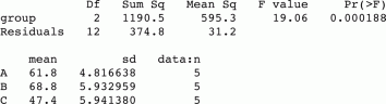
A traditional one way ANOVA results in the following output:

Regression model: score.num ~ group

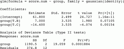
A regression model of score.num using group as an explanatory variable,results in the following output:

The one way ANOVA and the OLS regression model provide identical outputs. Both tests show an F-value of 19.06 and also show the differences between the groups. The intercept term for the regression model shows the mean value for the reference category (group A, 61.8), and the individual parameters show how different each group is from the reference; group B is seven units higher (i.e. has a value of 68.8) and group C is 14.4 units lower (i.e. has a value of 47.4)[6].

Dependent groups

In order to demonstrate the analysis of data collected using a repeated measures design (and a different number of groups), the following analysis compares just two of the groups reported in Table II – groups A and C. These data can be analysed using a paired t-test, or, equivalently, an OLS regression model.

Traditional test: paired t-test

In order to run a traditional paired t-test, the data need to be presented using a different structure (see Hutcheson, 2011b, for a discussion of data structures):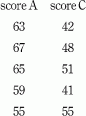

A traditional paired t-test results in the following output: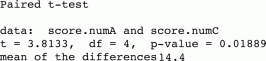

Regression model: score.num ~ group + subject

A regression model of a repeated measures design is identical to the dependent groups design, except that information about the subject is added to the model. This model requires each variable to be represented as a single column of data. The structure of the data in Table II is therefore appropriate and does not need to be changed.

An OLS regression model of score.num using group and subject as explanatory variables results in the following output: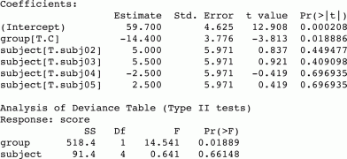

Although the results from the two analyses may look quite different, they are identical. Both techniques show the same significance for the group. The paired t-test value of 3.8133 is identical to the regression F-ratio of 14.541 (the square of the t-value is equivalent to the F-ratio;3.8133²=14.541) and both show the difference between the groups as being 14.4 units. The regression analysis, however, provides more information(for example, the significance of the subject variable) and also allows the option of including additional variables and computing a range of diagnostics.

B. Replacing the traditional non-parametric tests using regression

When the response variable is not continuous (or does not have a Gaussian distribution), a traditional non-parametric test can be used. There are a huge number of tests available (Siegal and Castellan, 1988) which can cause confusion for test selection. Many of the standard non-parametric tests can, however, be replaced with regression models (in this case, the proportional-odds model). The regression models reported here do not reproduce the non-parametric test results– they replace them (the statistics and significance levels are different). The following examples show the same analyses conducted on multi-category groups on ordered data collected from independent and dependent group studies.

Independent groups

A Kruskal-Wallis rank sum test or a regression model may be used to test whether there is a difference in “score.ord” (an ordered categorical variable) between the groups (indicated by variable “group”) for data collected using an independent-groups design.

Traditional test: Kruskal-Wallis rank sum test

A traditional Kruskal-Wallis rank sum test results in the following output:

• data: score. ord by group

• Kruskal-Wallis χ²=6.285, df=2, p-value=0.04317

Regression model: score.ord – group

A regression model of score.num using group as an explanatory variable results in the following output: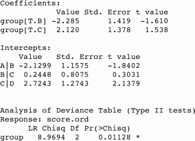

The traditional test shows a significant difference between the groups and a p-value of 0.04317. This is different to that provided by the regression model, which shows a p-value of 0.01128. Given the very small sample size, it is not appropriate to interpret these values with respect to the population. The regression model does, however, offer a number of advantages over the Kruskal-Wallis including the ability to test ordinality (the values of the intercepts provide clues about this) and the appropriateness of using an ordered regression model (this can be checked using the proportional-odds assumption test), the ability to add additional variables to the model and the availability of diagnostics.

Dependent groups

In order to demonstrate the analysis of data collected using repeated measures designs, the following analysis compares the ordered score data(variable “score.ord”) for the groups. These data can be analysed using a Friedman rank sum test, or a regression model.

Traditional test: Friedman rank sum test

In order to run a Friedman rank sum test, the data need to be presented using a structure similar to that used above for the paired t-test. A traditional Friedman rank sum test results in the following output:

• Friedman χ²=5.7333, df=2, p-value=0.05689

Regression model: score.ord ~ group+subject

A regression model of a repeated measures design is identical to the regression model used for the dependent groups design, except that information about the subject is added to the model. This model requires each variable to be represented as a single column of data. The structure of the data in Table II is therefore appropriate and does not need to be changed. A regression model of score.ord using group and subject as explanatory variables results in the following output: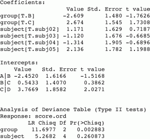

The Friedman test shows a difference between the groups equivalent to a p-value of 0.057. This is different to that provided by the regression model, which shows a p-value of 0.003. Given the very small sample size, it is not appropriate, however, to interpret these values with respect to the population. The regression model offers a number of advantages over the Friedman including the ability to test ordinality (the values of the intercepts provide clues about this) and the appropriateness of using an ordered regression model (this can be checked using the proportional-odds assumption test), the ability to add additional variables to the model and the availability of diagnostics.

C. Analysing categorical data using regression

The relationship between categorical variables is traditionally analysed using tests based on χ² that are applied to contingency tables. The statistics from these tests can, however, also be reproduced using generalized regression models which offer significant advantages over the traditional tests (for example, the ability to add additional variables into the model and the application of the same unified underlying theory for data analysis). A traditional contingency table analysis is compared to regression models using the data shown in Table II.

Traditional test

A contingency table analysis may be used to investigate the relationship between “group” and “region”. The contingency table derived from the data in Table II is:

A traditional contingency-table test results in the following output:

Regression models

There are two regression models that can be used to replicate the contingency table analysis provided above. Cell-count can be modelled using a GLM with a Poisson link (a GLM applied to count data), or one of the variables can be modelled using a GLM with a logit link (a GLM applied to unordered categorical data). Both of these are shown below.

A model of cell-count

The model used here predicts the cell-count using “group” and“region” as explanatories. The regression model is:

where the term “group* region” includes the main effects and the interaction (i.e. group + region + group:region). As we wish to assess the relationship between group and region, it is the interaction term between these that we are interested in. As the response variable is a count, we use a Poisson model which simply uses a log link between the response and explanatory variables. The model we run is therefore very similar to previous models except that a log link is used. A regression model of cell-count using group and region as explanatory variables results in the following output: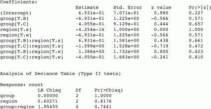

The interaction term in the Poisson model is identical to the G-squared statistic reported as part of a standard contingency table analysis. The Poisson regression model, however, provides a lot more information (for example, the comparisons between individual cells) and also allows the model to be extended with additional variables.

A model of an unordered categorical variable

It is also possible to replicate the contingency table analysis by directly modelling one of the unordered categorical variables. AGLM of the variable“group” is simply:

As the response variable is unordered categorical, we use the multinomial technique which automatically selects a logit link between the response and explanatory variables. The model we run is therefore very similar to previous models except that a logit link is used via the multinomial technique. A regression model of group using region as an explanatory variable results in the following output:The multinomial logit model “group ~ region” provides the same statistics as the Poisson model above (χ²=1.9546, which is also the same as that for the contingency table analysis). The multinomial model, however, offers a number of advantages, such as more detailed information about the relations between categories and the ability to add additional variables into the model (including variables measured on a continuous scale).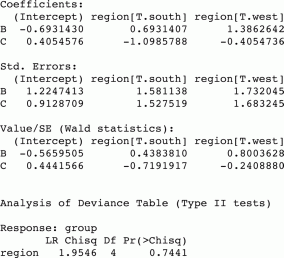

Conclusion

This tutorial has demonstrated that the traditional models for analysing grouped data may be represented or replaced by GLMs. The many seemingly different tests that cause so many difficulties for those learning statistics may be replaced by a single model:

Models of continuous, count, ordered and unordered categorical data, are all based on this same basic model. This model can be easily adapted to account for experimental design and also allows sophisticated diagnostics to be applied. The regression model also defines the variables needed to enter into the model and thereby provides the structure of the data, which is a difficulty commonly encountered by students. One of the biggest advantages to using GLMs, however,is the common underlying theory and the ease with which this can be taught.

Given these advantages, there seems little reason not to base statistical analysis courses on GLMs. It is time that test selection and teaching moved into the twenty-first century.

Graeme D. HutchesonManchester University, Manchester, UK, and

Les SchaeferIndependent Consultant, Hamburg, Germany

Notes

1. That is, identical results to those obtained using the traditional tests can be obtained using regression. As regression is far more flexible, the traditional tests are, essentially, redundant.

2. The link (~) for count data is the log – which equates to a log-linear model.

3. The application of dummy coding should not present any difficulty, as modern statistical packages automatically dummy code categorical variables (R Development Core Team, 2012).

4. Potentially confounding variables are controlled in the experimental design (random selection of subjects and random assignment to groups, etc.). Although such designs are assumed by traditional tests, they are rarely used in management research (most studies being survey-based).

5. These are just a few that are available.

6. Using regression, different dummy coding techniques can be used to provide different group comparisons. For example, a different reference category can be chosen, or each group can be compared to the mean of all groups (see Hutcheson,20 lie, for a discussion of dummy coding techniques).