Health monitoring of ground support system through point cloud processing: enhanced deformation analytics phase

Deep underground mining depends on consistent health monitoring of the underground environment to maintain safe working conditions and uninterrupted scheduled operation. Geostatic pressure results in drift deformation and, if left unchecked, may lead to the fall of roof strata. Deformation is the change in excavation geometry over time (Jones and Beck, 2018). To minimise deformation of the rock mass, kinematic analysis, numerical models and empirical techniques are used for ground support design (Jones and Beck, 2018). Ground support systems, such as rockbolts, are used to provide the tensioning support to the compressive strength of the rocks and help the rock to support itself (Bobet and Einstein, 2011). Ground support system is designed based on the structure and rock compressive strength and monitored post-installation to perform rehabilitation. Traditional deformation monitoring methods are based on manual point-to-point measurements performed using extensometers or instrumented ground support. However, local deformation is also affected by the ground support system through corrosion, yield and rehabilitation (Counter, 2014). Inadequate ground support will not provide sufficient compressive strength, and due to the dynamic nature of the strata, rehabilitation of ground support is a constant requirement. Hence, monitoring and rehabilitation of ground support are required to maintain safe working conditions in underground mines.

Monitoring the entire mine through manual inspection is impossible, and only damage mapping is performed through visual observations (Jones, 2020). Manual point-based inspection methods are inefficient, based on qualitative evaluation, and cannot be extended through automation. Light detection and ranging (LiDAR) enables the collection of spatial information through point cloud data (PCD). LiDAR retrieves information from the surroundings by transmitting a laser beam and capturing the reflection. Traditionally, in mining operations, LiDAR scanning has been performed as terrestrial laser scanning (TLS), which provides a detailed point cloud with high accuracy. However, TLS setup requires a static and stable setup, and cannot capture continuous surfaces due to occlusion, which increases the time required for the scanning process. Mobile laser scanning (MLS) utilises a combination of inertial measurement units and panoramic images to localise the moving scanner in 3D space. This capability is based on simultaneous localisation and mapping (SLAM) (Franzini et al., 2023). MLS can be carried out with handheld, vehicle or drone-mounted SLAM-enabled scanners. MLS enables scanning of large caverns with cavities and non-uniform surfaces. MLS has the advantage of providing spatially continuous coverage over extended distances, in GPS-denied environments (Jones and Beck, 2018). Due to a lack of absolute positioning, the collected point cloud must be transformed to the mine coordinates (local coordinate system used by the mine) during preprocessing.

PCD is generated from scanning performed using LiDAR devices. PCD is an unstructured data format, i.e. the structure of the stored data has no resemblance to the physical structure it represents (Liu et al., 2021). The PCD provides the position of each point as X, Y and Z coordinates. Additionally, the intensity value, which is based on the properties of the reflecting surface, is also stored. Hence, PCD processing requires adapting existing algorithms or developing new ones based on specific requirements.

The unstructured nature of PCD necessitates the development of techniques for extracting structural information. Popular methods for extracting structural information involve isolating a relevant set of points that are close to each other and computing eigenvalues to assess the distribution of points in space. These methods for extracting geometric features based on eigenvalues of point neighbourhood were pioneered by Pauly and Vandapel and extended by Weinmann (Pauly et al., 2003; Vandapel et al., 2004; Weinmann et al., 2015).

Various deep learning-based methods have been proposed for PCD processing, leveraging advances in image processing. However, due to the unorganised structure of the PCD, methods have focused on segmentation before processing. PointNet exploited the local structural invariance, and output the model with a similar transformation as the input, while utilising the symmetric set function (Qi et al., 2017). Deep learning methods have been explored for structural information extraction and the generation of PCD. The limitation of deep learning methods is that such methods require large amounts of labelled data for training and higher computational resources. Martínez-Sánchez extracted rockbolt information from construction sites using a deep learning technique with the purpose of co-registering successive scans before and after shotcreting (Martínez et al., 2012).

Mukupa et al. have presented an extensive review of PCD used for deformation monitoring of structures such as dams, tunnels, bridges, towers, beams, pipelines and land slope (Mukupa et al., 2017). Walton et al. presented a change detection method for underground excavations. They tested between fitting the tunnel cross-section to a rectellipse and a point-to-point comparison method (Walton et al., 2018). They reported that cross-sectional-based comparison to shape does not provide high accuracy due to (1) sensitivity to the placement of the shape with cross-section and (2) the excavation shape is highly irregular and hence cannot be captured with a regular shape. They concluded that the alignment process of two time-separated scans can significantly influence the apparent deformation, and hence, more quantitative methods should be developed. Similarly, other researchers have investigated the model fitting approach for bored civil tunnels with regular structure (Gosliga et al., 2006; Han et al., 2013; Yi et al., 2020). However, the excavation drill and blast method does not generate a smooth surface in mining drifts.

Jones examined cross-sectional excavation to compare deformation in mining drifts and concluded that the change detection algorithm should measure both magnitude and direction, and display the magnitude of change (Jones, 2020). However, this approach was based on manual inspection of PCD. Similarly, other researchers have explored cross-sectional deformation computation (Jiang et al., 2020; Kang et al., 2024). Since deformation is spread over the surface, such methods cannot generate information about the spread in relation to the ground support.

Deformation changes the tunnel surface over a period. Individual points in the PCD alone may not contain much information, but utilising the distribution of the point cloud can lead to better parameter estimates and deformation monitoring (Gosliga et al., 2006; Monserrat and Crosetto, 2008). Deformation analysis should quantify the spatial changes while distinguishing between convergence and divergence (Jones and Beck, 2018). Hence, a quantitative assessment of deformation should be performed over a period of time. Also, because the deformation effect is evident on the rockbolts, evaluating their protruding parts can offer a means for assessing rockbolt health and planning for ground support rehabilitation. This depends on developing methods to interrelate the condition of rockbolts and deformation. Patwardhan presents an overview of the automation of health monitoring of underground drift through point cloud processing (Patwardhan and Karim, 2024). Further, based on the overview, a detailed flow of PCD processing requirements for rockbolt information extraction in underground mines, considering various support structures, has been presented (Patwardhan and Karim, 2025).

The Wasserstein distance metric represents the optimal transportation problem between two probability distributions. The Wasserstein distance has applications in various fields, such as fluid mechanics, optimisation, computer vision, genomics, economics and finance (Panaretos and Zemel, 2019). Lai and Zhao proposed a method for point cloud registration utilising the Wasserstein distance. The approach for computing rotation invariant features using eigenvalues is applied in this work to reduce the effect of rockbolt orientation (Lai and Zhao, 2017). Garg et al. have demonstrated the applicability of the Wasserstein distance for quantification of ambiguous regions at object boundaries in the form of a loss function (Garg et al., 2020). Nguyen et al. present a systematic study on the use of the Wasserstein distance as a metric for comparison of point clouds (Nguyen et al., 2021). In this work, the Wasserstein distance is utilised to develop a method for quantifying changes in rockbolts and their surrounding surfaces over time. The quantification of change in rockbolts is achieved by computing Wasserstein's distance between two segments of a point cloud representing the same rockbolt, extracted from two PCDs acquired with a time gap between them.

Relative comparison of consecutive drift PCD is preferred since convergence and divergence both occur, and due to a lack of a global reference, a point of truth to compare two scans is difficult to ascertain. Quantitative representation of deformation extracted through spatially continuous PCD processing should support the generation of localised deformation rate and, in turn, integration with administrative controls like Digital Trigger, Action, Response Plans (TARPs). Hence, the purpose of this article is to propose a methodology for: (1) evaluation of point cloud quality before processing; (2) quantification of deformation through time-spaced PCD and (3) visualisation of the computed deformation to enable health monitoring and rehabilitation of the ground support system.

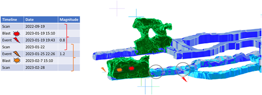
The data was acquired from a mining site located in the south of Sweden and was registered to the mine coordinate system with a depth marker of 1,241 m. Surveyors from the mining organisation carried out the data acquisition process. Several Lidar scans between 2022 and 09–19 and 2023–02–28 were performed and made available to be used for the development and testing of algorithms, as shown in Figure 1. However, only two scans were found to be useful for data processing purposes. This was mainly due to the low density of points or the large time difference between microseismic events and the scan time.

The methodology follows the following steps:

1. Selection of the region of interest

2. Point cloud quality assessment

3. Computation of spatial error

4. Computation of registration error

5. Computation of deformation

6. Rockbolt comparison–linear variation

7. Rockbolt comparison–volumetric variation

The data used for processing was collected using a BLK2GO scanner from Leica Geosystems (Leica, 2024) BLK2GO is a small handheld dual-axis LiDAR that supports MLS and can capture 420,000 point/s using a laser wavelength of 830 nm with a maximum range of 25 m. According to the manufacturer, the scanner is capable of an accuracy of 6 mm at 10 m and 8 mm at 20 m.

Popular data formats for PCD exchange are named as “las”, “laz” and “e57”. All these formats support storage of pointwise position information, intensity of reflection and colour associated with the point. Other features, such as point normal and point classification, can also be stored. In this project, the data made available was in E57 format with intensity values. The provided data was registered to the mine coordinate system.

Data processing and visualisation for this work have been carried out in Python programming language using Open3D library for point cloud processing support (Van Rossum, 1995; Zhou et al., 2018).

Human activity, such as blasting and excavation, causes disturbances that may lead to deformation in the mining drifts. Such activity data is important for selecting the region of interest for further data processing. Sensors record and triangulate the position of microseismic events occurring in the region surrounding the drifts. The data logs provide the location of the event in 3D space and the time of occurrence.

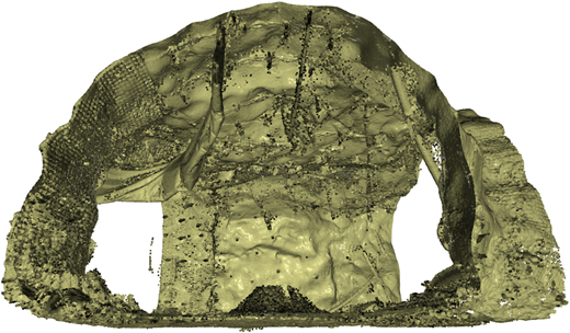
Figure 1 shows the details of the selection of a region of interest for processing. The blue areas represent the tunnels, and the green areas represent the post-blasting voids. The table shows the event data for blasting and recorded microseismic events with their magnitude. The cross symbols show the locations of the recorded microseismic events, where the locations of the highest magnitude of the two events are marked with a “thunderbolt”. The correspondence between the blast event, microseismic event and availability of LiDAR scan was evaluated to select the region of interest shown in circles. Finally, the intersection location of three tunnels (red thunderbolt) was selected as the test site due to the structural instability and the microseismic event due to previous blasting in the tunnel. The developed algorithms are independent of the selected region and can be applied to any other location. Figure 2 shows the 2D projection of the PCD of the selected region. This region is approximately 6 × 6 × 6m in size and is represented by about 32 million points. Ground support and rockbolts are visible on the walls and the ceiling, wire mesh on the left wall, and a deflated air circulation pipe near the ceiling.

The computation of deformation depends on comparing multiple point cloud datasets acquired over a period. As a first step, comparing the quality of PCD sets is required.

Point density is an essential feature of the PCD since it impacts every data processing step. High-density PCD acquisition is time-consuming, requires better hardware and surface properties, and requires high storage space and computational effort in the digital domain. A high sampling rate is not required for good quality sampling in all scenarios, as is well understood from information theory (Jerri, 1977). However, during PCD processing, point density is a critical factor for data processing algorithms and hence becomes important when comparing two or more PCDS. Point cloud density is evaluated by selecting a set of points (in this project, 1,500) that form the neighbourhood of a single seed point. The seed point is manually selected so the surface is relatively plane in the region. Point density is computed for the point cloud based on the region's volume.

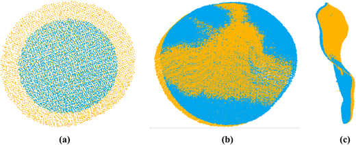
Figure 3 shows the samples of two-point clouds in blue and yellow colours with 1,500 points each. Figure 3 (a) shows samples in blue and yellow colours sourced from different LiDAR scanners. Their comparison shows that the point clouds occupy different volumes and hence have different point densities. Figure 3 (b) and (c) show front and side views of point clouds sourced from the same LiDAR device at different time intervals. Figure 3 (b) and (c) show that the datasets have the same point density since they occupy the same volume for 1,500 points. In addition, it can be observed that there is a slight misalignment between the two point cloud datasets.

Figure 3 (a) shows that PCDs can have different densities and hence different nearest neighbour distances. The point density can depend on the LiDAR device settings, raw data processing software, scanned surface, etc. Since density and nearest neighbour distances are required parameters to implement PCD processing algorithms, PCD evaluation is required for each individual dataset before processing. The PCD density can be matched by decimation.

Figure 3 (c) shows a small misalignment of the two surfaces; this may be caused by deformation or imperfect positional alignment of the two PCDs.

Such a comparison of point cloud quality provides:

1. A quick overview of the differences between the compared PCDs. This is required since the point density is required for the proper functioning of the rest of the algorithms.

2. The quality of registration. Since the surveyors carry out alignment using software tools, a small error is introduced while manually aligning marker points.

When the surfaces of two PCDs need to be compared, the data should be in the same 3D space with the least amount of error in positional alignment. In the case of underground drifts, a GPS-denied environment, the PCD lacks global alignment and should be aligned to a mine coordinate system. Transforming a PCD in 3D space that aligns with the used coordinate system is known as registration.

Registration can be performed by transforming the PCD according to the location of known markers (Arun et al., 1987). Marker-less registration is generally a two-step process where, first, a global registration is performed, followed by a local registration intended to reduce the registration error. However, this registration process is not perfect. It retains a minor registration error due to reasons such as, but not limited to, lack of absolute positioning, human error in marker selection, software limitations to transform the points correctly (local minima) and actual deformation of the marker positions. This minor error in registration is spatially variable and leads to the following issues:

1. The registration error leads to a mismatch in the six degrees of freedom, i.e. translations and rotations along the X, Y and Z axes.

2. If two PCDs are compared visually, the error combines registration error and deformation. Visual comparison has been used in the past, but it cannot provide any qualitative information, and is useable only when a high degree of deformation has occurred.

3. Since health monitoring of the ground support system requires integrating various data sources, a quantitative PCD comparison result is required.

As discussed in section 2, the PCDs are selected to be the closest before and after a microseismic event. The microseismic event is expected to generate deformation at various locations. However, due to a registration error, a straightforward distance computation between the surfaces will not provide the deformation value.

In this article, the smallest distance between two PCDs from the exact location will be called the spatial error. Equation 1 shows that the computed spatial error can be a combination of registration error and deformation at a given location.

The following approach has been developed to compute the spatial error. Lague et al. proposed an algorithm for comparison of complex topography called M3C2 (Multiscale Model to Model Cloud Comparison) (Lague et al., 2013). M3C2 has been adapted for 3D enclosing regions, and some implementation details have been changed to increase its efficiency in this context. The algorithm is described as follows:

1. A PCD is loaded and voxelisation (Patil and Ravi, 2005) is carried out. A voxel is a volumetric pixel and provides a mechanism to extract points in a neighbourhood. In this work, each voxel is a cube of side 0.4 m.

2. For the points of each voxel, which represent a small section of the tunnel surface, the following processing is performed:

   • The points' eigenvalues are computed, and the vector corresponding to the smallest eigenvalue is used as the perpendicular to the surface. This vector is called the surface normal.

   • A smaller cuboid of dimensions 0.05 × 0.05 × 0.5 m is created and aligned to the surface normal along the cuboid length and positioned at the surface as shown in Figure 5 

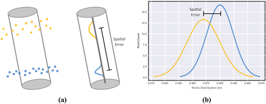
   • Points within the cuboid are extracted for the two PCDs being compared and projected on the surface normal as shown in Figure 4 (a) 

   • The difference between the peaks of the two distributions is used as the computed spatial distance at a location, as shown in Figure 4 (b) 

3. Step ii is repeated for two PCDs, hence computing spatial distance over the entire surface. Figure 5 shows the placement of point sampling cuboids along the surface of the drift

4. Histogram of spatial error is plotted to evaluate the distribution of spatial error

The result of the computation of spatial error at approximately 1700 locations out of 1921 had a spatial error <0.01 m, while the maximum value was around 0.04 m.

The spatial error has been computed at this stage, but both contributing factors, i.e. the deformation and registration error, are unknown. Deformation at a location can be computed if the local registration error can be ascertained.

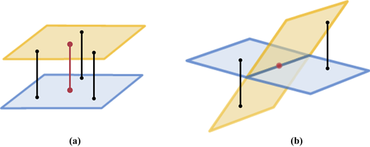
Figure 6 shows the possible scenarios causing registration error. The blue and yellow planes represent the surfaces from two PCDs used to compute deformation. The red point is the location where the registration error is to be computed, while the black dots are its neighbours. Figure 6 (a) shows the case when the two surfaces are almost parallel, and hence, the registration error is constant. Figure 6 (b) shows the case when the two surfaces intersect, and the registration error is variable.

The registration error at a given location can be computed by averaging the signed distance of the neighbours, i.e. the length of the black lines. The computed spatial distances of the neighbours provide the signed distances. Hence, the registration error can be computed as shown in Equation 2, where the registration error for point p is computed as the signed average of its n neighbours.

As shown in Figure 6 (a), the average of the black lines' lengths will be equal to the length of the red line; in Figure 6 (b), the two black lines will have equal values but with opposite signs, which will cancel out when averaged. Now, the deformation at a point p can be computed as the difference between its spatial and registration error, as shown in Equation 3.

The discussed method cannot ascertain the absolute registration error and will not completely remove the registration error, but it will reduce its effect locally. Better registration techniques, either through surveying or a better registration algorithm, can reduce the registration error and improve the quality of the computed deformation. After extracting the registration error from the two PCDS, the computed deformation is used to compare rock bolts on a one-on-one basis.

Failure of the rockbolt to provide ground support can happen when (1) the rockbolt loses its adhesion to the rock mass and moves freely along its length, (2) the rockbolt has been sheared in the rock mass due to lateral movement of strata, (3) the rockbolt plate is broken and the rockbolt is pulled inwards in the rock mass. Such failures of the rockbolt are visible on the protruding part of the rockbolt as a change in surface length or orientation, or a change in the rock surface in the close vicinity of the rockbolt. Two techniques to perform comparison of rockbolts from successive PCD have been developed, i.e. linear variation, focusing on the protruding rockbolt information, and (2) volumetric variation, focusing on the rockbolt and the region surrounding it.

A change in protruding rockbolts can indicate deformation in the rock mass, which may or may not be visible on the surface. Comparison of corresponding rockbolt information extracted from successive PCDs can be used as health monitoring information of the rockbolt and an indicator of deformation in the rock mass. The first requirement to compare rockbolts is the extraction of rockbolt information; this process has been carried out to export rockbolt information (Patwardhan and Karim, 2025). The following information is exported for each rockbolt:

1. A vector termed as surface normal, which is perpendicular to the drift surface where the rockbolt is present

2. A vector providing the orientation of the rockbolt

3. Angle between the rockbolt and the drift surface

4. The point where the rockbolt touches the surface

5. The point at the tip of the rockbolt

Corresponding rockbolts from two PCDs are paired by matching the position of the rockbolts on the drift surface. The length of an individual rockbolt is computed as the distance between the surface point and the tip point of the rockbolt. Change in length of the rockbolt is computed as the difference between the computed lengths of a rockbolt from two PCDs. It should be noted that the length of the rockbolt is computed between the surface and tip points and does not differentiate between rockbolt movement or surface movement; hence, the computed length difference itself is unaffected by the registration error.

Deformation at the rockbolt location also affects the surface in the close vicinity, which can result in the rockbolt plate or the shotcrete surface movement. Hence, a quantitative technique is required to compute the volumetric change to compare the overall variation in the rockbolt and surroundings. A volumetric measurement is suitable to accommodate the variations in the region surrounding the rockbolt. Figure 7 shows extracted points from two scans for the rockbolts; the misalignment is a result of registration error. A quantification method to compute a single value representing the change in the rockbolt and its surrounding regions can be used for health monitoring of the rockbolts.

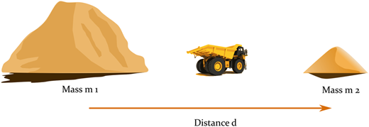
Wasserstein distance is the measure of dissimilarity between two distributions over a metric space, where the metric space provides a unit of measurement, and it is a statistical distance between two distributions (Panaretos and Zemel, 2019). It is also known as Earth mover's distance (EMD). Intuitively, it measures the effort required to move a given mass over the given distance, as shown in Figure 8.

Wasserstein distance is computed as shown in Equation 4. Where, $Ps,Pd$ are the source and destination probability distributions for which the Wasserstein distance $Wp$ is computed, the distance is computed between two points x and y such that the points are sampled from the distribution $γ$⁠. $γ$ belongs to the set of all the transport plans $Γ$ between the distributions $Ps,Pd$⁠. Finally, infimum extracts the optimal transport plan from the set of transport plans between the two distributions.

In this work, the Wasserstein distance has been applied to PCDs with similar point density. Hence, the computed value represents the minimum energy required to create the first set of points from the second set of points. This represents the overall variation in the region surrounding the rockbolt and includes deformation and registration error. Hence, the effect of registration error can be minimised similarly as discussed in section 2.2.

This work focused on generating quantitative deformation measurements for health management. To improve the utilisation of the results by rock mechanics engineers and other domain experts, visualisation of the results is required with the region's topography. This section presents screen captures of various visualisations created to represent the results of computations. Visualisations are in a 3D environment supporting interactive operations where the user can orient and scale to create a suitable point of view. The point cloud is augmented with colour and meshes such as bounding boxes, cones and spheres.

For clarity, the visualisations have been shown with a single computed feature, such as a change in rockbolt or deformation. However, multiple computed features can be visualised together to support health monitoring of a given location.

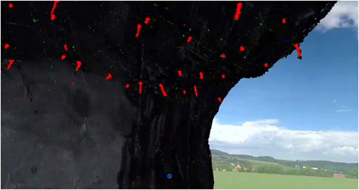
This result shows the PCD with modifications resulting from the computations in a virtual reality (VR) environment. Figure 9 shows a screenshot of PCD with detected rockbolts marked in red while the PCD is viewed in a VR environment. The VR environment has been created in the Azure remote rendering service (London, 2024). A VR environment can load PCD to create an interactive 3D health monitoring environment. The regions of interest in the PCD can be marked by colour or include shape meshes (e.g. spheres, bounding boxes, cones). Such visualisations can provide a visual comparative reference of the quantitative results of the computations over a given region and improve spatial awareness of local deformation while reducing the time of inspection. Such visualisation would allow the surveyors and rock mechanics engineers to perform off-site inspections by visualising the PCD remotely. Such visualisation, integrated with remotely operated vehicles, can be used for inspections of highly unstable areas, thus improving operational safety. Same PCD has also been used with augmented reality (AR) devices. Using AR allows the rock mechanics engineers to perform on-site inspections by projecting the results of computations onto the drift surface.

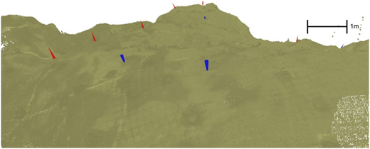
This result shows the visualisation of change in protruding length of corresponding rockbolts from two PCDs. Figure 10 shows the results of the comparison of rockbolts resulting from section 2.3.1. To perform the health monitoring, the surveyors scan the drift approximately once a month. Rockbolt information, such as rockbolt surface position on the drift, protruding length and angle to the surface, is extracted through PCD processing. Rockbolt counterparts are established by comparing the surface position and pairing the rockbolts between two subsequent PCDs of the exact location. Rockbolt protruding length comparison between the paired rockbolts is performed to compute any changes. The computed difference between the lengths is visualised as cones, where the length of the cone is proportional to the difference in protruding length, while the orientation and the colour of the cone represent the direction of movement. Figure 10 shows that the cones are placed at the rockbolt location and aligned with the rockbolts orientation. Cones in red colour show divergence and cones in blue colour show convergence; the orientation of the cones also indicates this. The visualisation uses perspective projection and hence represents the size of cones based on the distance from the viewpoint. The length of the cones has been scaled for visualisation.

However, the computation of the protruding length of the rockbolt is dependent on the surface detection near the rockbolt and the detected points on the surface of the rockbolt. Hence, small differences in the length of the rockbolt are rejected as measurement error. Since this computation is performed based on the drift surface to rockbolt tip distance, the computed difference in length is free from the effects of registration error. This result provides the position of change in protruding length of the rockbolt, but cannot differentiate whether the change is due to rockbolt movement or overall surface drift movement.

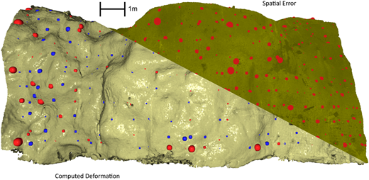
This result shows the visualisations generated from the computation of spatial error and deformation as discussed in section 2.2. Figure 11 shows the result of the computation error on the right and the final result of deformation computation on the left. The darker region on the right with red spheres represents the computed spatial error, while the lighter region on the left with red and blue spheres represents the computed deformation. The spheres are positioned at the location of computation, the sphere's colour represents the deformation red for divergence and blue for convergence, and the sphere's radius represents the computed deformation. The reduction in size of spheres between the two regions, i.e. spatial error and the computed deformation, indicates the removal of registration error. The shortcoming of this method is that the calculated deformation is relative to the surroundings. The visualisation uses perspective projection and, therefore, represents the size of spheres based on their distance from the viewpoint. The radius of the spheres has been scaled for visualisation.

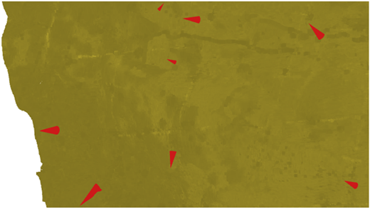
This result shows the visualisation of volumetric variation as discussed in section 2.3.2. Figure 12 shows the result of computing the Wasserstein distance between rock bolt counterparts. The result is represented with red cones, where the computed Wasserstein distance is represented by the length of the cone, and the vector formed between the two corresponding rockbolt tips is used to orient the cone.

The rockbolts are long metal rods and hence cannot change their position laterally on the drift surface. However, failure of the rockbolt to provide ground support can be indicated by the change in protruding length on the surface. It can be accompanied by a change in drift surface properties due to movement of the rockbolt plate on the drift surface or changes in the shotcrete surface. Computing the Wasserstein distance near the corresponding rockbolts provides a quantitative measure of variation in the region, including the rockbolt protruding length, variation in the rockbolt plate, and the surface near the rockbolt. This measurement estimates a volumetric change in the vicinity of rockbolts. Since the current mechanism of deformation computation is affected by the registration error, an improvement in the registration process through improved data preprocessing by the surveyors can improve the overall results.

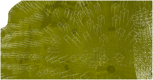
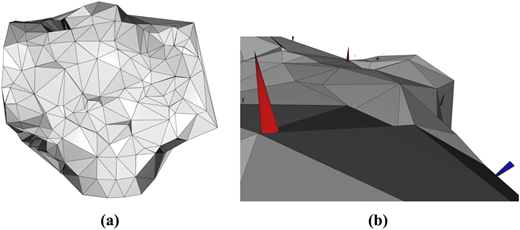
This result shows the visualisation of mesh representation generated using the rockbolt positions. Figure 13 (a) shows the surface mesh representation of the region of interest. The mesh nodes are the surface positions of the rockbolts, and the edges from a node connect to the closest neighbours of each rockbolt, without edge overlap. Figure 13 (b) shows a close-up view of the surface mesh with the results of the comparison of rockbolts with the cone lengths representing the computed change in length, while the colour and the orientation represent the direction of change to the surface.

The advantage of representing the surface as a mesh is in terms of required space, visualisation and accuracy of representation. The PCD of the same region requires about 700 MB of storage, while the mesh representation requires a few 100 KB, reducing the storage space requirement. The mesh representation can be visualised interactively through various general-purpose software tools as well as in web browsers. This can reduce the storage and computation burden for the end user and enable handheld devices for information consumption and inspection remarks. Since the mesh is generated using the extracted positions of the rockbolts on the surface, it maintains a high degree of accuracy in the representation of the surface. The edges in the mesh provide the inter-rockbolt distances, and the regularity of the triangular pattern can be used to evaluate the condition of the rockbolts as a system to provide ground support.

This article proposes a methodology for quantifying the deformation of underground mining drifts through point cloud processing and other data sources to support health monitoring and, in turn, integration with Digital Trigger, Action, and Response Plans (TARPs).

Underground drift PCD collected through LiDAR devices can have varying properties in terms of point density and scanning pattern. Hence, an initial data quality evaluation is required to extract the parameters related to a PCD and use them for future processing. PCD point density represents the point neighbourhood distance, which is critical for clustering algorithms.

PCD collected in a campaign-based manner is used to quantify the deformation. However, since underground drift has a global movement and forms a GPS-denied environment, an absolute relative positioning in 3D space is unavailable without a time-consuming surveying exercise. This introduces minor imperfections in the alignment of the two or more PCDs, generally known as registration error. Hence, the computed spatial error combines deformation and the registration error. The method for the computation of spatial error is based on the M3C2 algorithm and adapted for 3D space. Adaption of M3C2 to 3D space allows the computation of the spatial error for the tunnel instead of a cross-sectional region. An averaging-based method has been used before the visualisation stage to reduce the effect of registration error while retaining the deformation information. This has shown a marked reduction in spatial error. Improvements in the surveying methodology can lead to a reduction in the registration error.

To use rockbolt position comparison as one of the indicators of deformation in the rock mass, comparison of rockbolts information has been performed. Visualisation of the computed change in rockbolt protruding length supports the rockbolt health condition evaluation. This is possible since the change in rockbolt protruding length indicates possible failure of function in the rockbolt, i.e. due to loss of adhesion in case of length increment and 2) surface layer deformation in case of length decrement.

The rockbolt and the face plate act as a system providing ground support to the surrounding rock mass; hence, a methodology for comparison of the surface surrounding the rockbolt counterparts was required. Wasserstein distance is the minimal effort required to reconfigure one distribution to another. The rockbolt and its close vicinity were used as the distribution. The computed Wasserstein distance value was used as the magnitude of volumetric variation. This provides a quantitative result for comparison of the surface variation, including the rockbolt, surface plate and the rock surface and can be a valuable indication of overall rockbolt condition.

Finally, the computation results are presented as visualisations to be used by rock mechanics engineers to evaluate the condition of the rockbolt and perform rehabilitation. As shown in this article, the possibility of visualisation of point clouds augmented with colours and meshes in VR and AR can improve the inspection process while reducing the time and safety requirements.

Deep underground mines are geologically dynamic environments where both gradual and abrupt changes can occur due to movements in rock mass, ground support failure, or human activities such as blasting and excavation. Maintaining a safe working environment and adhering to the planned schedule are extremely important. The safety of operations is ensured through regular inspections conducted via both manual and automated methods. Surface scanning, such as with LiDAR, has facilitated automation and helps in capturing information from large areas. However, comparing deformation over time and quantifying these results has not received significant attention. Therefore, this article presented methodologies to generate quantifiable results regarding changes in rockbolts and deformation over a period.

Quantifying linear and volumetric changes in rockbolts, along with surface deformation from PCD collected during campaigns, empowers domain experts-including rock mechanics engineers-to perform health monitoring of ground support. Furthermore, adding more point cloud datasets over time can facilitate the extraction of the rate of deformation in individual regions, aiding in the development of improved rehabilitation strategies for ground support. Visualising the outcomes using virtual and AR devices further enhances the representation of information.

Rockbolt failure, deformation, and surface cracks are four-dimensional entities spread over three physical dimensions and time. The presented methods work in these four dimensions. However, the resolution is limited due to the registration accuracy during data preprocessing. Surveyors can easily address this shortcoming when the data is collected for this specific purpose.

PCD is used for structural monitoring, but it cannot detect small surface failures such as cracks. Future work will focus on developing methodologies to monitor surface cracks in the dimensions of space and time.