An improved model for building energy consumption prediction based on time-series analysis

D(m)

distance between x_i and x_p in the embedding dimension m

d_i, y_i

Euclidean distance to the centre point

d_min

minimum value of d_i

d(x_i)

Euclidean distance of the new initial vector

e_t

residual part

F(x,y)

kernel function

h_t

output information of the state unit

l

time step

m

best dimension calculated

$ṁ2,t$

corrections of the first- and second-order momentum terms

N

total sample size of the observation data

P_i

weight of y_i

r

artificially set critical value

t

delay time of the time series

t

embedded dimension constructed for the new sequence

w_t

weight

w_X, w_Y

values of weights

X

reset gate outputs of the gate recurrent unit (GRU)

X

input matrix

X(r_i)

ith vector

x, y

independent variables of the kernel function

x_i

delay vector

x_p

adjacent point of the delay vector after phase space reconstruction

Y

update gate outputs of the GRU

Y

output matrix

Y_i

linear part in x_i

y_i

vector set

Z_i

non-linear part in x_i

α, β

undetermined coefficients where the square error is the smallest when the weighted least square method m = 1 is used

γ

system growth rate

ϕ

learning rate

The building energy consumption of renewable energy refers to the energy consumption of off-site renewable energy resources at the construction site. Since the era of industrialisation, the overexploitation and utilisation of energy have led to vicious problems such as resource shortage, global warming and environmental pollution. Against this background, the development and utilisation of renewable energy and green energy is imminent (Othman et al., 2021). The determination of the proportion of renewable energy is a difficult problem in the integration of renewable energy into buildings. Some scholars have developed software programs for the selection of building energy. The results showed that the new renewable energy proportion optimisation method has a good effect on reducing the natural gas consumption, power consumption and cost of buildings (Aliabadi et al., 2021). The research of Zygmunt and Gawin (2022) showed that the use of renewable energy in the renovation of buildings and the use of the energy cluster mode could effectively reduce the energy consumption of buildings, save electricity and reduce carbon dioxide emissions. In the process of building renovation and reduce carbon dioxide emissions, Coimbra (2021) used renewable energy to reduce energy consumption.

The effective use of building energy is one of the effective measures to reduce building costs and protect the environment. The utilisation of renewable energy in buildings is one of the important directions of renewable energy utilisation, because the energy consumption of buildings occupies a considerable proportion in the urban energy structure (González-Arias et al., 2022). To make buildings use energy scientifically, it is necessary to plan for energy use – that is, to have accurate predictions of building energy consumption (Hamada et al., 2022). In building energy consumption prediction, time-series analysis is a targeted technique because energy consumption data usually show certain regularity and trends (Phan et al., 2020). In addition, support vector machines (SVMs) and related neural networks have also been studied and utilised more in data processing and prediction, which are mature technology relatively (Lan et al., 2019). This research proposes a building energy consumption prediction model of renewable energy based on chaotic time series combined with an improved SVM neural network, to improve further the accuracy of energy consumption prediction in this field. In the field of energy consumption prediction, many researchers have made contributions. Pan et al. (2022) proposed an energy consumption prediction system based on a generative adversarial network for the problem of energy consumption prediction in workshop processing. Relatively accurate predictions could still be made in the context of missing data. In response to the energy consumption of global data centres, Liu et al. (2020) proposed an energy consumption prediction model based on global data centre traffic and power usage efficiency. Doroodi and Mokhtar (2019) noticed that some industries emit too much greenhouse gases (GHGs) and conducted trend analysis and exponential smoothing analysis of the energy consumption of each energy sector. The results showed that industry had the highest GHG emission among the demand industries. The results had important contributions to the design of current environmental protection strategies.

In terms of time-series analysis and the development and application of SVM technology, Khan et al. (2022) conducted a time-series analysis of the data on natural soil abrupt change in a certain area. They also provided a model for the application of time-series analysis to land cover issues. Sulaiman and Juarna (2021) conducted a time-series analysis of the unemployment rate in Indonesia based on an autoregressive integrated moving-average model and distinguished factors related to the unemployment rate, including urbanisation, industrialisation, demographic education and minimum wages. The results of the study showed that the model they developed could predict unemployment more accurately. In response to the economic slowdown, Kim (2021) established an economic forecasting model using vector autoregressive models and time-series data of long- and short-term interest rates. Furthermore, he made predictions of redemption interest rate, loan interest rate and treasury bill interest rate data. The model had a high reliability after a t-test and a significance test of cross-correlation matrix. For the detection of obstructive sleep apnoea, Valavan et al. (2021) proposed a heart rate signal derivation model combined with the SVM grid search algorithm. The experimental results showed that the recognition accuracy of the model for obstructive sleep apnoea exceeded 80% (Valavan et al., 2021). Chen et al. (2021) developed a mathematical optimisation-based SVM machine learning optimisation model that can analyse field workflows for improved drilling operations with high accuracy. Essam et al. (2022) noticed the negative impact of suspended sediments in rivers and rivers on water quality and proposed a water-suspended sediment load prediction model based on an SVM and an artificial neural network. The performance test of the model showed that the model showed good performance in different data sets highest sediment load prediction accuracy.

The aforementioned research results showed that the time-series analysis method and SVMs had better data prediction performance in different fields. However, according to the collation of the latest research results in the fields of energy consumption prediction, time-series analysis and SVMs, it was found that there were not many predictions in the field of building energy consumption prediction for renewable energy. There was also a certain research gap in the direction of combining building energy consumption prediction of renewable energy with time series and SVMs and other complex technologies. To improve the energy consumption prediction of renewable resources in the construction field, the time-series analysis method and SVMs were selected to predict the building energy consumption in this research. In this prediction model, the chaotic time-series model could predict the change in building energy consumption linearly. Moreover, the gate recurrent unit (GRU)–SVM prediction model was used to process the non-linear residual part of the chaotic time-series prediction to improve further the accuracy of the chaotic time-series model. The author hopes that the new model can be used to bring practical results to this field.

Based on time-series analysis, the building energy consumption prediction model uses the technology of chaotic time series and SVM prediction. The role of chaotic time-series modelling is to predict the building energy consumption change of renewable energy linearly. Meanwhile, the SVM prediction model is used to process the non-linear residual part of chaotic time-series prediction to improve the accuracy further. The reason for using this design is that although chaotic time-series analysis has good prediction accuracy in linear prediction of energy consumption, its non-linear residual part has a weak processing ability. Therefore, the SVM model is introduced to predict this part.

Traditional time-series analysis models and summation autoregressive moving-average models are able to analyse the building energy consumption of renewable energy and predict with certain accuracy, but their prediction accuracy is very limited (D’Urso et al., 2016). This is because the factors affecting the building energy consumption of renewable energy are many and complex. The obvious factors affecting energy consumption include seasonal factors, climatic factors, regional factors and industrial factors. Some of these factors show a certain periodicity, but the comprehensive effect of various factors still makes the building energy consumption prediction of renewable energy more difficult and complex. In addition, the combined effects of other factors such as industry development and population changes also have a significant impact on changes in building energy consumption. Furthermore, they further strengthen the chaos of energy consumption data. Since the energy consumption data themselves have multiple characteristics of periodicity, aperiodicity and chaos, it is necessary to judge the nature of the sequence before time-series analysis (Bencherif et al., 2021). Here, the Lyapunov maximum exponent is used to judge the properties of time-series data. First, the observed data sample matrix is reconstructed, and the reconstructed matrix vector is shown by the formula

In Equation 1, X(r_i) represents the ith vector, t is the delay time of the time series and m is the embedded dimension constructed for the new sequence. Let the total sample size of the observation data be n; then, the reconstructed new matrix is m × n dimensional. After that, the first vector is taken as the starting point. Furthermore, there is a need to search for the vector closest to the starting point among all the vectors as the end point to set an initial vector. The distance between vectors is calculated as the Euclidean distance. The next step is to calculate the system growth rate of the new initial vector, and the calculation process is shown in the formula

In Equation 2, γ is the system growth rate, l represents the time step and d(r_i)represents the Euclidean distance of the new initial vector. There is a need to continue to set up vectors and calculate their distances according to this rule until all phase points are calculated. Then, all growth rates should be averaged to obtain an approximation of the Lyapunov exponent. Finally, the input dimension should be increased and the calculation repeated until the output value no longer has a significant difference with the change of the dimension m. At this time, the output value at this time is the Lyapunov maximum exponent. In the chaotic time series, the delay time has a significant impact on the phase space reconstruction of the time series and the actual output results of the time-series analysis, so the choice of delay time must be careful. Here, the minimum mutual information method is used to confirm the delay time of building energy consumption prediction. The mutual information function relationship of the minimum mutual information method is shown in the formula

In Equation 3, A and B represent two time series. According to the correlation conditions generated by b_k in time series B, whether the condition information is generated by a_i in time series A can be known. Then, the average mutual information between the two time series can be obtained. After the functional relationship is clarified, the sample space is divided into multiple modules, and the number of points in each module is calculated as its probability. Finally, the first minimum point in all modules can be used as the delay time.

Besides the delay time, the embedding dimension of the chaotic time-series analysis model is also an important parameter. When the embedding dimension is too small, the phase space will collapse, which will make some points that should be far away from each other become very close. This seriously affects the calculation accuracy. When the embedding dimension is too large, the amount of data that need to be processed in the actual calculation process of the model will increase significantly. Thereby, it can significantly increase the computational complexity, which will reduce the computational effectiveness of the model. At the same time, operating pressure and noise interference will seriously affect the performance of the model. Here, the pseudo-proximity point method is used to solve the problem of embedding dimension. This method starts to debug the time-series analysis model with a smaller embedding dimension. When the current time-series model is too small, the distance between non-adjacent points is narrowed, resulting in the phenomenon of pseudo-adjacent points. The embedding dimension is continuously adjusted. When the number of pseudo-neighbouring points is the smallest, the corresponding embedding dimension is considered to be available. The mathematical process of embedded dimension judgement is shown in the following formulae:

In Equations 4 and 5, x_i represents the delay vector and x_p represents an adjacent point of the delay vector after phase space reconstruction. D(m) is the distance between the two in the embedding dimension m, and r is an artificially set critical value. When [D(m + 1) − D(m)]/D(m) is greater than the critical value, this means that D(m) changes greatly with the embedded dimension – that is, x_i and x_p are pseudo-proximity points. The embedding dimension is continuously increased until the time-series model does not satisfy [D(m + 1) − D(m)]/D(m) > r. Then, the embedding dimension at this time can be used as the best dimension. In the construction of chaotic time-series prediction and model, the common methods include the weighted local method, global prediction method and local prediction method, among which the prediction accuracy of the weighted local method is usually higher than those of the other two methods. The weighted local method is also used in the building energy consumption prediction model of renewable energy in sequence analysis. In the weighted local method, the centre point selects the last point of the phase space trajectory and uses the phase points around the centre point as reference points to establish a local reference vector set, where the vector set is expressed as y_i. (i = 1, 2, 3, …, q) The weights of y_i points can be defined as shown in the formula

In Equation 6, α and β are undetermined coefficients where the square error is the smallest when the weighted least square method m = 1 is used, as shown in the formula

In Equations 7 and 8, d_i is y_i, the Euclidean distance to the centre point; d_min is the minimum value of d_i; and P_i is the weight of y_i. The partial derivatives of α and β in J should be found and simplified. Then, the following formula can be obtained:

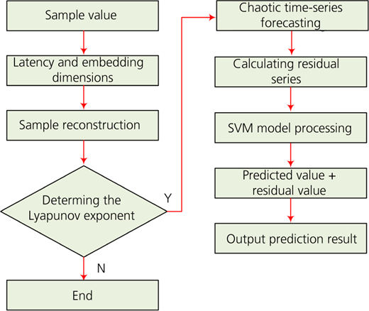
The energy consumption prediction formula based on chaotic time-series analysis can be obtained by substituting Equations 9 and 10 into y_i+1 = αe + βy_i. A flow chart of the building energy consumption prediction model of renewable energy based on time-series analysis is shown in Figure 1. In the chaotic time-series process, the delay time and embedding dimension are calculated after the samples are input. Then, the samples are reconstructed, and the Lyapunov index is calculated. The chaotic time-series results are the output according to the calculation results.

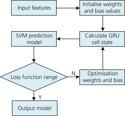
In the building energy consumption prediction model of renewable energy based on time-series analysis, the role of the SVM prediction algorithm is to deal with the non-linear part of the energy consumption data through the calculation of the residual, because the non-linear part of the chaotic time-series analysis cannot be better forecast. The SVM prediction algorithm used here is the GRU–SVM algorithm, which combines the GRU and the SVM. Among them, GRU is an improved feedforward neural network whose recurrent unit contains only two gates. Compared with long short-term memory (LSTM), GRU has higher learning efficiency and can solve well the gradient disappearance and gradient explosion problems of feedforward neural networks under long-term data dependence (Jia et al., 2020). The reason for choosing an SVM was that this model has a strong search ability and can efficiently classify samples compared with other models and search for the optimal classification hyperplane (Zhu et al., 2020). These properties make SVMs have a strong ability to obtain the global optimal solution and could avoid the local extreme value problem. The running process of the GRU–SVM algorithm is shown in Figure 2. After the feature is input, the network will initialise the weights and bias values. After the GRU cell state is counted, the GRU–SVM network will iterate continuously. When the result meets the requirements of the loss function and the set threshold, it can output the results.

When designing the GRU part, the Adam algorithm is used to improve the standard GRU structure. The Adam algorithm is an extended stochastic gradient descent algorithm, which is characterised by the consistency of the learning rate – that is, the learning rate remains unchanged during the operation of the algorithm. At the same time, the Adam algorithm can significantly improve the speed of gradient update with only a small increase in system memory usage. The output information after GRU combined with the Adam algorithm is shown in the following formulae:

In Equations 11–13, X and Y represent the reset gate and update gate outputs of the GRU, respectively. In addition, h_t represents the output information of the state unit at time t. w_X and w_Y are the values of both weights. x_t is the input information at the current moment. In the hidden layer of the neural network, the output expression of GRU shows that the data dimension of the algorithm and the number of nodes will change according to the change in the data set. In the process of improving the GRU model by using the Adam algorithm, the parameters of the GRU model are updated by the gradient estimation of the first and second moments to get rid of the interference of the gradient transformation and increase its stability. The iterative process after GRU combined with the Adam algorithm is shown in the formula

In Equation 14, w_t is the weight of the tth iteration and ϕ represents the learning rate. $ṁ1,t$ and $ṁ2,t$ represent the first-order and second-order momentum term values, respectively. Their definitions are shown in the following formulae:

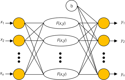
In Equations 15 and 16, α and β are the estimates of the exponential decay rates of the first and second moments, respectively, while $ṁ1,t$ and $ṁ2,t$ represent the corrections of the first- and second-order momentum terms. SVMs are a binary classifier. Thus, when using SVMs to deal with problems containing more than two features, it is necessary to build an SVM-based multi-classifier (Bai et al., 2022). Building energy consumption prediction of renewable energy is a multi-feature problem, because many influencing factors need to be considered. For these problems, the multi-class construction of SVM classifiers is used to deal with each feature one to one. In the specific operation, each type of data is combined with other types of data in pairs, and an SVM classifier is set for each combination. When classifying, a vote is needed in each classification for the target data. The category with the most votes is considered the correct category for the data. This multi-class construction mode can effectively reduce the amount of test data to speed up training. A schematic diagram of the model of SVM combined with the GRU network is shown in Figure 3. The model contains m units; the first m − 1 units are GRU units; each GRU unit has its own state and input; and finally, all data are processed and output by SVM.

After completing the construction of the SVM forecasting algorithm, it is used to model the building energy consumption forecasting activity of renewable energy. First, the energy consumption time series is divided into two modules: linear autocorrelation and non-linear correlation, as shown in the formula

In Equation 17, x_i represents the chaotic time series and Y_i and Z_i represent the linear part and the non-linear part in x_i, respectively. After modelling the Y_i part based on the chaotic time series, the mathematical expression of the residual is obtained as

e_t in Equation 18 represents the residual part. By using SVM modelling for the residual part, the residual sequence is obtained as shown in the formula

In Equation 19, n is the total sample size of the observed data and m represents the best dimension calculated. According to the residual sequence, the input and output matrices of the building energy consumption residuals of renewable energy can be obtained, as shown in the following formulae:

In Equations 20 and 21, X and Y represent the input and output matrices, respectively. Finally, the kernel function of SVM is selected. The kernel function expression is

In Equation 22, x and y are the independent variables of the kernel function. The internal structure of the SVM for non-linear problems is shown in Figure 4. There are n kernel function units in the structure, and its role is to map samples to high-dimensional space to solve multidimensional problems.

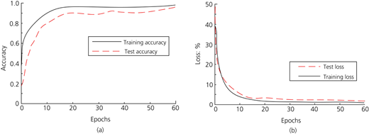
The building energy consumption prediction model of renewable energy is composed of the GRU–SVM neural network and chaotic time series. Therefore, the performance test of the energy consumption prediction model is also divided into two parts. The first is the performance test of the neural network, and the second is the algorithm performance test of the neural network combined with chaotic time series. The performance of chaotic time series is evaluated. The observed results of the accuracy and loss values of the GRU–SVM model during training and testing are shown in Figure 5. The data used for performance test in the experiment come from the relevant data on energy in the statistical yearbook.

Figure 5(a) shows the accuracy test results of the GRU–SVM algorithm during training and testing. It can be seen that the training accuracy curve of the algorithm has a maximum accuracy of 98.3%, and it is relatively stable. The test set accuracy curve is stable at 97.2%. Figure 5(b) shows the loss performance of the GRU–SVM algorithm in the training and test sets. Among them, the training set loss value is at least 1.5%, and the corresponding test set loss value is at least 4.1%. The accuracy gap between the test set and the training set is only 1.1%, and the gap between the loss values is also small. This performance shows that the GRU–SVM model has higher prediction performance and better generalisation ability and has the potential to be put into practical use. The trained GRU–SVM model is evaluated in terms of model accuracy and error, and the results are shown in Figure 6.

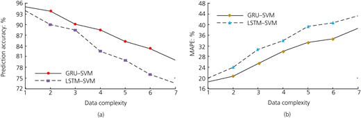
In this experiment, the GRU–SVM algorithm and the comparison algorithm are tested and compared in a data set with no complexity. The comparison algorithm is the LSTM–SVM algorithm. Because LSTM and GRU are the same type of network, they can be comparable. Figure 6(a) shows the accuracy comparison results. The prediction accuracy of the two algorithms decreases with the increase in the complexity of the data set. However, the accuracy curve of the GRU–SVM algorithm is always above that of the LSTM–SVM algorithm, which is shown in each data set. The accuracy of GRU–SVM is higher than that of LSTM–SVM. GRU–SVM has the highest accuracy of 95.5%. The accuracy gap between the two shows an increasing trend with the increase in data complexity, and the difference is up to 7.6%. Figure 6(b) shows the comparison results of the errors of the two algorithms, and the mean absolute percentage error is used as the evaluation index. The error curves of the two algorithms show an increasing trend with the increase in data complexity. The highest error of GRU–SVM is 38.1%, while that of LSTM–SVM is 43.6%, and the difference is 5.5%. After completing the evaluation of the GRU–SVM algorithm, the next step is to evaluate the performance of the chaotic time-series prediction model combined with the neural network. First, the accuracy of energy consumption prediction of the model in the sample data is evaluated, and the results are shown in Figure 7.

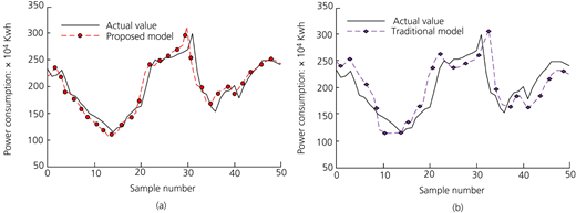
Figure 7(a) shows the test results of the energy consumption prediction model, and Figure 7(b) shows the prediction results of the traditional model. Compared with the real energy consumption data, it is found that both models can fit the trend and trend of the energy consumption data curve well, which shows that the two models have a certain predictive ability. From the image, the curve of the energy consumption prediction model is obviously closer to the real curve, while the curve of the traditional model is farther away from the real curve. This shows that the prediction results of the energy consumption prediction model are closer to the real situation. The energy consumption prediction model deals with the residual of energy consumption data. Compared with the traditional model, this is one of the improvements of the energy consumption prediction model. Therefore, this part needs to be investigated in the performance evaluation. The inspection results are shown in Figure 8.

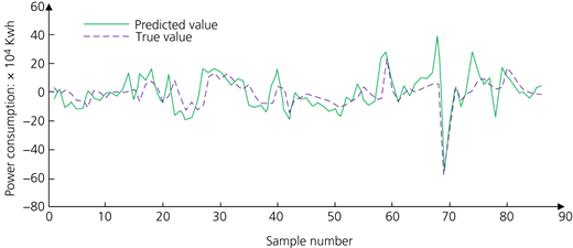
Figure 8 describes the difference between the residual calculated by the energy consumption prediction model in the sample data and the actual error value, and it can be seen that the predicted value curve and the actual value curve fit closely. The minimum difference between the two curves is 0 – that is, they are exactly the same. The maximum difference is only 311 000 kWh, which is relatively small for energy consumption data. After the analysis of residuals is completed, it is necessary to compare the overall prediction error of the energy consumption prediction model. The comparison results are shown in Table 1.

In Table 1, the indicators used to measure the prediction error of the model are the mean absolute error and the mean relative error. The traditional SVM model, LSTM model, chaotic time-series model and ordinary time-series model are used as comparison models. Analysing Table 1, it is found that the mean absolute error of the energy consumption prediction model is 7.25, which is the lowest among all the tested models. The mean absolute error values of the models other than the energy consumption prediction model are distributed between 9.6 and 10.2, which are significantly higher than that of the energy consumption prediction model. From the point of view of the average relative error, the average relative error of the energy consumption prediction model is 4.13%, which is also the lowest among the models used in the test. The average relative error of the chaotic time-series model is second only to that of the energy consumption prediction model, with an error value of 5.52%. The average relative error of the chaotic time-series model is 1.39% higher than that of the energy consumption prediction model. After a comprehensive performance test of the energy consumption prediction model, the model can be tested with real renewable energy building energy consumption data, which can confirm the performance of the model in actual use. The test results are shown in Figure 9.

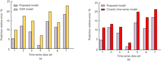
Figure 9(a) shows the comparison results between the energy consumption prediction model and the traditional SVM model. Figure 9(b) shows the results of the energy consumption prediction model and the chaotic time-series prediction model. The energy consumption prediction model is composed of the improved SVM model and the chaotic time-series model, so the two original models are selected as the comparison objects. A total of seven data sets are used for comparison. It can be seen that the average relative error of the energy consumption prediction model in each data set is smaller than those of the two comparison models, which once again shows that the design of the model is effective. In the fourth time-series data set, the energy consumption prediction model exhibited the lowest average relative error of 2.3%. The average relative error of the traditional SVM model in the same data set is 6.8%, and that of the chaotic time-series model is 4.1%, which are significantly higher than that of the energy consumption prediction model.

The research, utilisation and development of green energy and renewable energy are the focus of energy reform and energy structure transformation around the world. The energy consumption of buildings cannot be ignored in the current energy consumption structure, so the design of renewable energy for buildings is necessary. Because the time-series analysis method and SVM have good performance in data prediction, the time-series method and SVM are innovatively combined and used to establish the prediction model of building energy consumption. The prediction model is a building energy consumption prediction model based on GRU–SVM and chaotic time series. In this prediction model, the chaotic time-series model can predict the change of building energy consumption linearly. To improve further the accuracy of the chaotic time-series model, the GRU–SVM prediction model is used to process the non-linear residual part of the chaotic time-series prediction. After the performance test of the energy consumption prediction model, it is found that the GRU–SVM part of the training accuracy curve of the model has the highest accuracy rate of 98.3%, and it is relatively stable. The test set accuracy curve is stable at 97.2%, and the accuracy gap between the test set and the training set is only 1.1%. Among the partial prediction errors of GRU–SVM, the model error is the highest at 38.1%. The prediction error of LSTM–SVM used for comparison is 43.6% at this time, and the difference between the two is 5.5%. In the verification of the overall prediction ability of the energy consumption prediction model, it was found that the average absolute error of the energy consumption prediction model was 7.25, and the average relative error was 4.13%. Compared with those of other comparative models, the average absolute error and average relative error of the energy consumption prediction model are the lowest. Comprehensive analysis of the information given by the test results shows that the model has a considerable performance improvement in energy consumption prediction compared with other traditional prediction models. The experimental results show that the chaotic time-series model can accurately predict the change in building energy consumption. Furthermore, the GRU–SVM prediction model can further improve the accuracy of the chaotic time-series model. However, there are still deficiencies in this study. Although the model can predict energy consumption in real data sets, it has not been verified using real-time data. At the same time, the data anomalies caused by abnormal consumption demand were not considered in the model design process, so these factors should be included in the model research in the follow-up study.