


This study aims to explore the impact of just-in-time (JIT) arrival systems on the attractiveness and economic viability of short sea shipping (SSS), particularly in the feeder containership sector. Specifically, it quantitatively examines how the optimization of sailing speeds (occurring from the application of JIT systems) may influence the competitiveness of SSS, especially in terms of cost.
Within a vector error correction model framework, we conduct scenario analysis to assess the influence of speed optimization on freight rates. The dataset includes the Intra-Asia Container Freight Index, average speed and fleet development of feeder ships.
The results suggest that the implementation of a JIT arrival policy leads to moderate freight rate reductions, ranging from −0.18% to −4.39%. Beyond the cost benefits, speed optimization through virtual arrival policies enhances the overall competitiveness of SSS in terms of transit time, service reliability and environmental footprint.
To the best of our knowledge, this study is the first to investigate the impact of JIT arrival systems on the competitiveness of SSS while also providing empirical evidence. The findings suggest that policymakers and relevant stakeholders should embrace JIT systems to render SSS a more competitive and sustainable mode of transport.
1. Introduction
Modern supply chains are characterized by increasing complexity, with efficiency of operations, cost reduction and sustainability playing a major role. In this context, short sea shipping (SSS) – defined as the transport of cargo over short distances, i.e. without crossing an ocean – seeks to enhance its integration into intermodal transportation systems.
Coastal transport, especially in areas with archipelagic geography, such as Southeast (SE) Asia, is vital for domestic and regional trade. In the SE Asia peninsula, shippers mainly use SSS or trucking (Chang and Thai, 2017), while air transport is another option (though less popular in the case of cargo transport). Feeder traffic, a subset of SSS, plays an important role in this area, connecting major transshipment hubs, such as Singapore and Tanjung Priok, to smaller regional ports.
While SSS is a vital link of the hub-and-spoke network in SE Asia, feeder vessels are confronted with significant challenges stemming from poor facilities and inefficient operations of some regional ports. Long waiting times and unpredictable delays are major issues for shippers, driving them to alternative modes of transport whenever feasible. From a policy-making perspective, there are efforts to improve connectivity, notably from the Association of Southeast Asian Nations (Arof and Zakaria, 2020). Tackling the challenges of SSS requires collaboration among key stakeholders, as well as the adoption of new technologies and practices toward more efficient supply chains.
In recent years, just-in-time (JIT) systems and associated virtual arrival (VA) policies have attracted attention in the maritime industry. JIT is originally a management strategy that minimizes inventory and waste by coordinating the delivery of raw materials with production schedules. The equivalent strategy in the maritime sector pertains to the drastic reduction of port congestion by adjusting sailing speeds. The typical method of berth management in tramp shipping, which is based on the “first-come, first-served approach,” results in ships arriving at the port unnecessarily early and waiting until a berth becomes available. On the other hand, the arrival of feeder ships (which operate under liner transport services) is mostly based on fixed schedules linked to the arrival time of large containerships. However, feeders may still rush to ports due to the competition for limited berths and pressure to match the schedule of mother ships, avoiding delays. In both the case of tramp and liner services, unnecessary rushing to arrive early is a key contributing factor to port congestion, which in turn affects the efficiency of wider supply chains. From the perspective of shippers, this is perceived as a weakness of SSS in general, undermining the efforts toward its more extensive integration in logistics chains.
The effectiveness of traffic management systems depends on transparent communication between vessels and port authorities, reliable technologies and collaboration among all stakeholders involved, such as ship operators, charterers and port authorities. The role of shipbrokers could also be critical (Tsioumas et al., 2023). Ineffective coordination and unstructured ship-to-port communication during the ship arrival process pose significant challenges to the adoption of JIT systems in shipping (Veenstra and Harmelink, 2022). Furthermore, the lack of reliable and accurate information on costs and savings may hinder the broader uptake of VA policies (Rehmatulla and Smith, 2015). Addressing these challenges is critical for the effective adoption of JIT systems in shipping.
This article focuses on the impact of implementing JIT arrival policies in the feeder traffic of SE Asia. Specifically, it quantitatively explores how the optimization of sailing speeds (occurring from the application of JIT systems) may influence the competitiveness of SSS, especially in terms of the cost. The current body of literature has mainly focused on the impact of JIT arrivals on fuel consumption and emissions. Motivated by the ongoing effort – at the policy and academic levels – to enhance the competitiveness of SSS, this study aspires to expand the relevant literature by exploring how the adoption of this emerging technical solution, rooted in the JIT philosophy, may affect the key competitive dimensions of SSS, notably cost.
2. Literature review
A longstanding domain of interest in maritime logistics, SSS offers the potential to minimize the carbon footprint of global supply chains (Mustakim et al., 2025) and improve (among other parameters) air quality (El-Zeiny et al., 2025), all within the overarching objective of sustainable operations (Batista Santos and Santos, 2024; Izdebski et al., 2024). Towards this end, the body of research has employed a wide range of methodologies, including Geographic Information Systems (Karountzos et al., 2024), time series analysis (Abuella et al., 2025), propulsion power allocation (Vergara et al., 2025), pre-gate concepts (Krüger et al., 2025) and benchmarking (Costa et al., 2024). These methods have a wide range of applicability, from ferries (Mayanti et al., 2025) and high-speed crafts (Martínez-López et al., 2024) to autonomous (Ahmed et al., 2024; Laryea and Schiffauerova, 2024) and hybrid (Barone et al., 2024) ships and container terminals (Bartosiewicz et al., 2024), fuel prices (Ollila et al., 2024), crane operations (ter Haar et al., 2024) and relevant case studies (Santos and Santos, 2024).
SSS offers important advantages compared to land transport, such as lower greenhouse gas (GHG) emissions, alleviation of congestion on road networks, safety and flexibility (Paixão and Marlow, 2002; Medda and Trujillo, 2010). In particular, the environmental and social benefits of SSS have been recognized by policymakers to such an extent that they financially support SSS as a viable alternative to road transport (Suárez-Alemán, 2016; Psaraftis and Zis, 2020).
However, SSS faces serious challenges that inhibit its competitiveness and viability. These include port inefficiencies (Ng, 2009; Suárez-Alemán et al., 2014), low frequency of services, lack of reliability in terms of departure and arrival times and complex administrative procedures (Paixão and Marlow, 2002; Medda and Trujillo, 2010).
The selection of the most suitable mode of transport is a decision-making problem; as such, it depends on relevant criteria. The consensus in the literature is that the prevailing mode selection criteria comprise cost, frequency of services, transit time, punctuality and safety (Papadimitriou et al., 2018). Paixão and Marlow (2002) point out that additional inventory costs and the value of time make shippers opt for unimodal transport over intermodal or multimodal forms. While cost remains a critical factor, many studies emphasize the growing importance of quality, including reliability, on-time delivery and frequency of transport (McGinnis, 1990; Lu, 2003; Fanam et al., 2018). Interestingly, Meers et al. (2017) reported that price and transit time have similar impacts on modal shift potential. According to Beuthe and Bouffioux (2008), modal choice is also affected by qualitative factors, such as distance, type and value of goods. They also estimate the relative weight of each attribute in decision-making and for container transport, they find that cost is the most important factor (71.4%), followed by transit time (9.7%), reliability (6.9%), flexibility (4.7%), frequency (4.1%) and safety (3.2%).
Also, although environmental criteria are gaining more attention than in the past, they remain less influential compared to cost and service quality, especially for smaller shippers (Van den Berg and De Langen, 2017). McKinnon (2014) states that although many shippers measure CO2 emissions, very few make decisions based on this. A shift to more environmentally friendly modes of transport requires policy measures and incentives in the form of subsidies (Tao et al., 2017). Sustainability as a mode selection criterion is expected to become more relevant in the face of new regulations that affect transportation costs, such as the Emissions Trading System (ETS), the Energy Efficiency Existing Ship Index and the carbon intensity indicator. These measures have been introduced by the International Maritime Organization (IMO) in the context of the 2023 IMO GHG Strategy, aiming at reducing the average GHG emissions per transport work across international shipping by at least 40% by 2030, compared to 2008 (IMO, 2023).
The prioritization of the mode selection criteria may differ depending on the characteristics of each region. Chang and Thai (2017) examine the shippers’ choice behavior in SE Asia and find that cost and time are the most important determinants, while some shippers may focus on other factors, such as service quality, customer relationship and CO2 emissions.
The implementation of JIT systems and related VA policies promises to optimize sailing speeds, thereby reducing congestion and emissions (Arjona Aroca et al., 2020). This further aligns SSS with decarbonization efforts in the maritime industry (Stavroulakis et al., 2023; Prousaloglou et al., 2025). Importantly, these traffic management systems may offer additional benefits that are relevant for SSS, as they address key competitive dimensions, such as cost and timely delivery.
The JIT philosophy was initiated in Japan during 1950s and gained increasing popularity when Toyota successfully implemented it in its automotive production system (Monden, 2011). JIT is based on elimination of waste, continuous improvement and pull production (Shingo, 1989; Hitomi, 2017).
Supply chain management offers fertile ground for the application of JIT principles. The effective application of JIT relies heavily on appropriate coordination among all actors of the supply chain in order to ensure on-time delivery of the right number of raw materials (Fullerton et al., 2003). The ultimate goal is to achieve effective and efficient flow along all supply chain stages and improve responsiveness to customer demands. This highlights the high reliance of JIT supply chains on transportation systems (Morash and Clinton, 1997). The weaknesses of SSS, especially the delays, create bottlenecks that are often the reasons for the preference for alternative modes of transport.
In this context, maritime logistics, including SSS, can benefit from the JIT philosophy, provided that it is adapted to the special characteristics of this business. Mubder (2024) posits that a JIT arrival system, enabled by a pre-booking berth allocation policy, should synchronize the arrival time of ships with the operating times of cargo handling systems in the port. This is expected to minimize port waiting times and offer cost advantages while improving the port connectivity with the hinterlands. Lind et al. (2021) state that JIT should be combined with time slots for berthing and data sharing to achieve optimal outcomes.
Feeders are mainly used for the movement of containers between regional markets and major hub ports. Efficiency is crucial for transshipment hubs, which are served by feeders within hub-and-spoke networks (Lee and Jin, 2013). The efficient operation of feeder networks determines the viability of the underlying supply chains. This also influences the attractiveness of feeders over alternative modes of transport – on routes where they are available. Therefore, the analysis of the success factors of feeder services can be linked to the wider scope of the competitiveness of SSS.
As mentioned, the main benefits of JIT and VA policies are the reduction of fuel expenses and GHG emissions, respectively. Despite the plethora of studies on the latter (Du et al., 2015; GEF-UNDP-IMO Global Maritime Energy Efficiency Partnerships Project and Global Industry Alliance to Support Low Carbon Shipping, 2020), we mainly focus on the impact on the economic aspect, as it is more related to the scope of our quantitative analysis.
The study by IMO-Norway GreenVoyage2050 Global Industry Alliance (2020) estimates that the implementation of a JIT system in containerships can offer an average fuel consumption savings of 14.16% when the speed is optimized over the entire voyage, 5.90% when optimized over the last 24 h and 4.23% under the last 12-h scenario. Those results are consistent with an older study conducted in the context of the MONALISA project (2010-EU-21109-S), which calculated a 10–12% reduction in the bunker bill. In another study, Jia et al. (2017) found that fuel savings can range from about 7% under the scenario of a 25% reduction in port congestion to 19% if congestion is eliminated.
While the quantification of the expected impact on fuel expenses is valuable, it does not necessarily provide an accurate indication of the corresponding freight rates. It is well-documented that despite the close link between freight rates and fuel expenses, the formation of freight rates requires additional considerations (Munim and Schramm, 2017). In this context, our study undertakes to explore how JIT arrivals may affect freight rates rather than fuel expenses.
3. Data
The dataset for this study includes the Intra-Asia Container Freight Rate Index, reflecting the freight rates of feeder ships in SE Asia; the fleet development of feeder containerships with a capacity of 100–2,999 TEU, corresponding to the supply of feeders and the average speed of feeders.
All data were extracted from Clarksons Research Shipping Intelligence Network and comprised monthly time series from January 2016 to June 2024.
We first inspect our time series to detect any signs of potential seasonality. For this purpose, we performed seasonal-trend decomposition using LOESS. This method decomposes a time series into three constituent components: trend, seasonal and residual. Focusing on the seasonal component, we can check for recurring patterns that reveal seasonality. Figure 1 illustrates the seasonal decomposition plots of each variable.
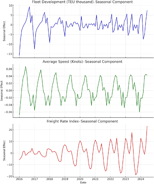
It is observed that the time series “fleet development” and “average speed” do not exhibit strong seasonality, as the fluctuations are mostly random, without any clear pattern. On the contrary, the Intra-Asia Container Freight Rate Index shows clearer periodic fluctuations, revealing the presence of a seasonal component.
Seasonality can lead to misleading model estimates, creating spurious relationships. Therefore, we de-seasonalize the Intra-Asia container freight rate index so that the model captures the actual dynamics of the data. The seasonal adjustment of this series is accomplished using the X12-ARIMA method in EViews. This widely used statistical procedure, developed by the United States Bureau of the Census, is based on regression-ARIMA models to account for outliers and other distorting effects and eventually perform seasonal adjustment of the time series (Findley et al., 1998).
Table 1 shows the descriptive statistics for the variables of this study during the period under consideration.
Descriptive statistics
| Freight rate index | Average speed | Fleet development | |
|---|---|---|---|
| Mean | 93.2591 | 13.50255 | 4351.116 |
| Q1 | 60.56551 | 13.29 | 4095.099 |
| Median | 65.73199 | 13.515 | 4238.613 |
| Q3 | 108.7928 | 13.74 | 4552.929 |
| Maximum | 231.844 | 13.86 | 5137.369 |
| Minimum | 39.23862 | 13.13 | 4009.37 |
| Std. dev | 52.39742 | 0.223774 | 313.9736 |
| Observations | 102 | 102 | 102 |
Source(s): Table by authors
These descriptive statistics provide insight into the data characteristics and the variability in the SE Asian feeder sector. The high standard deviation of the Freight Rate Index (52.4) is indicative of high variation from its mean (93.3). In contrast, the standard deviations of fleet development and average speed suggest moderate and low variability, respectively. Therefore, the sampled data indicate that feeder freight rates fluctuate considerably, whereas their average speed and their fleet capacity exhibit more moderate changes.
Table 1 also reveals the likely existence of outliers – specifically high extreme values – in the Freight Rate Index, as the mean (93.3) exceeds the median (65.7), indicating a positively skewed distribution. This is also evidenced by the high discrepancy between the third Quartile Q3 (108.8) and the median (65.7). In contrast, there are no indications of outliers in average speed and fleet development, as their distributions appear more symmetrical, without large differences among the first Quartile (Q1), median and the third Quartile (Q3).
4. Modeling framework
4.1 Cointegration
Two or more (individually) non-stationary time series, integrated of the same order after differencing, are said to be co-integrated if there is a stationary linear combination among them (Engle and Granger, 1987). This implies the existence of a long-run equilibrium with short-run adjustments.
Correction of short-term deviations from the long-term equilibrium is achieved through an error correction mechanism.
In this study, we check if the variables are cointegrated using the Johansen cointegration test (Johansen, 1988).
4.2 Vector error correction model (VECM)
The vector error correction model (VECM) is an unrestricted version of vector autoregression (VAR), incorporating an error correction component. This term accounts for the speed of adjustment to the long-term equilibrium after a change in an independent variable. VECM models are suitable for non-stationary but cointegrated time series. This modeling framework is suitable for analyzing time series data that share a long-term equilibrium relationship while also capturing their short-term dynamics. Essentially, the VECM is an extension of the VAR model by adding an error correction term (ECT) that accounts for the speed of adjustment. The modeling of cointegrated time series using this approach is well-documented in the literature (Granger, 1981; Engle and Granger, 1987). It has also been applied in various time series-based studies in the field of maritime transport (e.g. Kavussanos and Nomikos, 2003; Coto-Millán et al., 2005; Tsioumas and Papadimitriou, 2018).
The mathematical representation of the VECM model (Granger, 1981; Engle and Granger, 1987) is as follows:
where yt is a vector of all n variables at time t, Δyt are the first differences of each variable, Π is the cointegration matrix representing the ECT (corresponding to the long-term relationship), Γi (for i = 1, …, n) are matrices capturing the short-term dynamics (i.e. the effect of changes in the lagged values of a variable on all others) and εt is a vector of error terms.
5. Results
5.1 Model specification and diagnostics
In this study, we develop a VECM model after testing the variables for stationarity and cointegration. The Intra-Asia Container Freight Rate Index is used as the dependent variable and all other variables as explanatory.
We first apply the Augmented Dickey–Fuller (ADF) test of stationarity. The statistical properties of non-stationary time series change over time, leading to spurious regressions, unless they are co-integrated. The cointegration implies the existence of a long-run equilibrium relationship among non-stationary variables. According to the output in Table 2, all variables are non-stationary at their levels but stationary in first differences.
ADF test
| Levels_p-value | First differences_p-value | |||||
|---|---|---|---|---|---|---|
| Intercept | Const. and trend | None | Intercept | Const. and trend | None | |
| Freight rate index | 0.5115 | 0.6660 | 0.1150 | 0.0000*** | 0.0000*** | 0.0000*** |
| Average speed | 0.8213 | 0.5156 | 0.3724 | 0.0000*** | 0.0000*** | 0.0000*** |
| Fleet development | 1.0000 | 0.9992 | 0.9719 | 0.6954 | 0.0000*** | 0.6067 |
Note(s): *** indicates rejection of the null at 1% level, **at 5% and * at 10%
H0: the series is non-stationary, H1: the series is stationary
Source(s): Table by authors
Based on the findings of the stationarity test, we check for the existence of co-integration, since all variables are integrated of order 1, i.e. I(1). We select one lag based on the Schwarz Information Criterion, and then, we apply the Johansen Cointegration test.
Table 3 indicates that there is one cointegrating relationship at the 0.05 level. This confirms the existence of a long-term stable relationship among freight rates, fleet development, and speed, despite their short-term deviations.
Johansen co-integration test
| Variables | Lags | Hypothesized No. of CE(s) | Trace | 0.05 CV (trace) | Max Eigenvalue | 0.05 CV (Max Eigen.) |
|---|---|---|---|---|---|---|
| Freight rate index – Average speed; fleet development | 1 | None* | 32.03085 | 29.79707 | 26.36826 | 21.13162 |
| At most 1 | 5.662591 | 15.49471 | 4.863995 | 14.2646 |
Note(s): * denotes rejection of the hypothesis at the 0.05 level
CV: critical value, CE: cointegrating equation
The tests assume a restricted intercept in the co-integrating equation and no deterministic trends in the series
The trace statistic tests H0: r cointegrating relations against H1: k cointegrating relations
The max eigenvalue statistic tests H0: r cointegrating relations against H1: r+1 cointegrating relations
Source(s): Table by authors
Therefore, we can use a VECM model for the three cointegrated variables in this study. Table 4 reports the outcome of the most important residual diagnostic tests for this model.
Residual diagnostics
| Diagnostic test | Null hypothesis | p-value | Decision |
|---|---|---|---|
| LM test for autocorrelation | No autocorrelation in residuals | 0.82 | No rejection of H0 |
| Portmanteau test | No autocorrelation in residuals | 0.82 | No rejection of H0 |
| White Heteroscedasticity test (with cross terms) | No heteroscedasticity | 0.76 | No rejection of H0 |
Source(s): Table by authors
Serial correlation (or autocorrelation) occurs when the error terms of a regression model are not independent of each other. Heteroscedasticity refers to data for which the variance of the error terms is not constant over time. Although the presence of autocorrelation and/or heteroscedasticity does not lead to biased estimates, it undermines the reliability of hypothesis tests for the statistical significance of the regression coefficients.
Table 4 shows that the null hypothesis of no autocorrelation in residuals in both the Lagrange multiplier (LM) test and the Portmanteau test is not rejected (p-value 0.82) at a 5% level of significance. Also, the White Heteroscedasticity test fails to reject the null hypothesis of homoscedasticity (p-value 0.76) at a 5% significance level, indicating that there is no heteroscedasticity in residuals. Overall, the diagnostic tests indicate that there is no evidence of serial correlation and heteroscedasticity in the VECM model used in this study. Therefore, the model is well-specified, with no significant problems. It should be noted that the results of these diagnostic tests also imply that the potential outliers (identified based on Table 1) do not distort the model’s reliability.
This VECM model is then used for scenario analysis, investigating the percentage change in freight rates under different scenarios of reduction in the average sailing speed. Given that VA policies typically cause a downward adjustment of sailing speed, this study aims to offer a quantifiable measure of the impact of such policies on freight rates.
5.2 Scenario analysis
Eventually, we use the VECM model we developed to shed some light on how JIT arrivals affect freight rates in the feeder market. Speed optimization driven by VA policies essentially leads to a reduction in the average sailing speed. Our methodology examines the impact of different scenarios of speed reduction in the freight rate index.
The baseline speed of 13.5 knots corresponds to the mean value of the feeder speeds in our dataset. This speed is reduced by up to 25%, and we examine the freight rate change for each scenario. We do not expand the analysis beyond the 25% reduction, because a speed of 10 knots would result in extremely late arrivals, making it an impractical option for feeder ships (IMO-Norway GreenVoyage2050 Global Industry Alliance, 2020).
Table 5 indicates a negative response of freight rates to speed reductions, with decreases ranging from −0.18% to −4.39%. As the speed goes down, the changes in freight rates become larger. The decline in freight rates could be attributed to lower transport costs, which arise from lower fuel consumption. However, in maritime transport, the elasticity between fuel cost and freight rates is relatively low (Brancaccio et al., 2023). This may partly explain the low sensitivity of freight rates to speed changes. Another contributing factor could be related to the improved attractiveness of feeders – driven by better quality of services – which in turn strengthens the bargaining power of feeder operators. This counteracts the downward pressure from lower transport costs.
Scenario analysis
| Speed reduction (%) | Speed (Knots) | Freight rate index impact | Freight rate index impact (% Change) |
|---|---|---|---|
| 0 | 13.5 | 93.2591 | 0% |
| 1% | 13.365 | 93.09521 | −0.18% |
| 2% | 13.23 | 92.93133 | −0.35% |
| 3% | 13.095 | 92.76745 | −0.53% |
| 4% | 12.96 | 92.60356 | −0.70% |
| 5% | 12.825 | 92.43968 | −0.88% |
| 6% | 12.69 | 92.2758 | −1.05% |
| 7% | 12.555 | 92.11191 | −1.23% |
| 8% | 12.42 | 91.94803 | −1.41% |
| 9% | 12.285 | 91.78415 | −1.58% |
| 10% | 12.15 | 91.62026 | −1.76% |
| 11% | 12.015 | 91.45638 | −1.93% |
| 12% | 11.88 | 91.2925 | −2.11% |
| 13% | 11.745 | 91.12861 | −2.28% |
| 14% | 11.61 | 90.96473 | −2.46% |
| 15% | 11.475 | 90.80085 | −2.64% |
| 16% | 11.34 | 90.63696 | −2.81% |
| 17% | 11.205 | 90.47308 | −2.99% |
| 18% | 11.07 | 90.3092 | −3.16% |
| 19% | 10.935 | 90.14531 | −3.34% |
| 20% | 10.8 | 89.98143 | −3.51% |
| 21% | 10.665 | 89.81755 | −3.69% |
| 22% | 10.53 | 89.65366 | −3.87% |
| 23% | 10.395 | 89.48978 | −4.04% |
| 24% | 10.26 | 89.3259 | −4.22% |
| 25% | 10.125 | 89.16201 | −4.39% |
Source(s): Table by authors
The magnitude of freight rate changes is relatively small but noticeable, so there are far-reaching implications. From the perspective of the competitiveness of feeder services (and more generally SSS), the speed optimization through JIT arrivals addresses several mode selection criteria. As mentioned in Section 1, cost efficiencies enhance feeder ships’ competitiveness against alternative transport modes. However, according to some studies, the modal shift from road to sea is more likely when SSS rates (including land rates) are at least 35% lower than the cost of road transport (Paixão and Marlow, 2002).
Other key selection criteria include transit time and on-time delivery. The speed reduction due to JIT arrivals may initially give the false impression that the total transit time will increase. Yet, this is not accurate; what increases is the sailing time and not the total transit time. In fact, if a VA policy is widely adopted in a specific region, the total transit time could potentially be reduced due to lower idle time in port, which offsets the longer sailing. Also, the reduced port congestion improves the punctuality of feeder services, removing a serious bottleneck in their supply chain.
Finally, speed optimization aligns with recent efforts to reduce the environmental footprint of ships, thereby enhancing the competitiveness of SSS.
6. Conclusion
This study sheds some light on the impact of JIT arrivals on the competitiveness of SSS. Focusing on the SE Asian feeder market, we examined how sailing speed optimization – stemming from VA policies – affects freight rates. This scenario analysis was based on the VECM modeling framework. The results suggest that as the average speed of feeder ships decreases, freight rates fall moderately. This is mainly attributed to lower transportation costs – a key determinant for the formation of freight rates – as well as to the enhanced bargaining power of feeder service providers.
Despite the seemingly modest impact on freight rates, the implementation of JIT policies also affects other critical aspects of the competitiveness of SSS. Speed optimization reduces unpredictable delays – a major challenge in maritime logistics, making SSS more reliable and punctual. Furthermore, virtual arrivals improve the environmental sustainability of SSS. Although the environmental footprint has not been a priority for shippers, new regulations, such as ETS, are expected to increase the importance of environmental criteria. Speed optimization stemming from JIT arrivals reduces emissions, aligning SSS with the decarbonization goals outlined in the International IMO GHG Strategy. While JIT alone is not sufficient to meet such ambitious targets, it is a critical operational measure that complements broader efforts toward green maritime logistics.
The findings of this study highlight the importance of supporting the wider adoption of JIT systems in maritime transport as a way to foster the competitiveness and sustainability of SSS. The relevant stakeholders, such as shipping lines, shippers, port authorities and policymakers, should coordinate their efforts to ensure the seamless integration of JIT arrivals, promoting a more sustainable and efficient SSS. Specifically, port authorities could invest in innovative digital platforms, such as Pronto (initially tested in the ports of Rotterdam, Algeciras, Felixstowe and Houston), which allows information exchange about port calls in real time, facilitating JIT arrivals. Additionally, investments in Port Community Systems and artificial intelligence-based predictive analytics are equally important for streamlining data sharing across various stakeholders and forecasting berth availability. Shipping lines can benefit from JIT systems not only through lower fuel expenses and alignment with decarbonization goals but also because short-haul maritime transport becomes more competitive against trucking.
Despite its contributions, this study is subject to certain limitations, which provide opportunities for future research. First, the analysis focuses on SE Asian feeder traffic. Despite the increasing importance of intra-Asian trade in recent years, the results may not fully capture the dynamics of other regions. In future studies, it would be interesting to explore the effect of JIT systems in other SSS corridors, such as in the European Union (Motorways of the Sea), in the US and Africa. Additionally, expanding this approach to other sectors beyond containers could provide valuable insights. Finally, while this research is based on monthly time series, future studies could enhance the precision of the analysis by utilizing higher-frequency data (e.g. daily) or even automatic identification system data, subject to availability.
A previous version of this paper was presented at the XXV International Conference on Material Handling, Constructions and Logistics (MHCL) 2024, which took place in Bar (Montenegro) from the 12th to the 14th of December 2024. The present paper has benefited from the comments of the conference participants.

