This paper aims to examine containership routing and speed optimization for maritime liner services. It focuses on a realistic case in which the transport demand, and consequently the collected revenue from the visited ports depend on the sailing speed.
The authors present an integer non-linear programming model for the containership routing and fleet sizing problem, in which the sailing speed of every leg, the ports to be included in the service and their sequence are optimized based on the net line's profit. The authors present a heuristic approach that is based on speed discretization and a genetic algorithm to solve the problem for large size instances. They present an application on a line provided by COSCO in 2017 between Asia and Europe.
The numerical results show that the proposed heuristic approach provides good quality solutions after a reasonable computation time. In addition, the demand sensitivity has a great impact on the selected route and therefore the profit function. Moreover, the more the demand is sensitive to the sailing speed, the higher the sailing speed value.
The vessel carrying capacity is not considered in an explicit way.
This paper focuses on an important aspect in liner shipping, i.e. demand sensitivity to sailing speed. It brings a novel approach that is important in a context in which sailing speed strategies and market volatility are to be considered together in network design. This perspective has not been addressed previously.
1. Introduction
The demand for sea transport has continuously grown during the past few decades. Nearly 80% of worldwide trade is transported on water (UNCTAD, 2016). Moreover, maritime transportation can be classified into one of three general modes: industrial, tramp and liner operations. In particular, liner shipping operates according to a schedule on fixed routes between specific ports based on timetables. It transports approximately 16% of the world’s goods loads in tons (Branchini et al., 2015). In addition, various decision levels, including strategic, tactical and operational, exist in liner shipping. Strategic decisions include network design, alliance strategy and fleet size and mix. Tactical decisions involve fleet deployment, speed optimization, schedule construction and frequency determination, and operational decisions include cargo booking, cargo routing and rescheduling (Meng et al., 2014).
This paper addresses a combined strategic and tactical problem of integrated containership routing, speed optimization and fleet sizing. We assume that the decisions regarding the fleet mix and ships' size are already made. Most liner companies guarantee weekly service calls at each port included in the service (Cheaitou and Cariou, 2017). A single vessel deployed in a liner service cannot serve long-distance routes while satisfying the weekly service frequency of all the ports in the service, mainly because of the limitation in sailing speeds (Cheaitou and Cariou, 2012). Reducing the number of vessels deployed in a service can reduce operating costs. Consequently, containership routing, speed optimization and fleet sizing decisions are related and have a significant impact on the operational efficiency of liner companies. The containership routing problem, which consists in choosing the ports of call and their sequence while considering the revenues that may be collected from each visited port, is similar to the travelling salesman problem with profit (TSPP) (Toth and Vigo, 2014), but with special liner transportation properties related to the multiple vessels to be deployed in the service. One of the formulations of the TSPP that is called the Profitable Tour Problem (PTP) is the closest to the one adopted in this paper.
In the literature of maritime transportation, several studies focus on containership routing (Christiansen et al., 2013; Meng et al., 2014). For example, Liu et al. (2011) address both container routing and ship deployment and cargo routing problems at a tactical level. The authors propose a joint optimization model and sequential model formulations for comparison with an objective to maximize the shipping capacity utilization considering empty container repositioning. More generally, most of the works on liner shipping service modelling and optimization consider a fixed sailing speed (Gelareh et al., 2010; Meng and Wang 2011a, 2011b; Wang et al., 2011; Wang and Meng, 2011; Song and Xu, 2012).
Moreover, many papers have investigated the optimization of the vessels' sailing speed. For example, Wang and Meng’s (2012b) show that the third power relationship between the bunker consumption and the sailing speed can be used if not enough historical data are available. Cheaitou and Cariou (2012) develop a direct liner service model for a slow-steaming strategy between two ranges of ports to identify the optimal speed for cases in which perishable products are affected by time while frozen and dry products are not. Others investigated exact solutions approaches (Hvattum et al., 2013) or heuristic approaches (Castillo-Villar et al., 2014). However, the literature on sailing speed has been developing with may related works in the last few years (Cariou and Cheaitou, 2014; Andersson et al., 2015; Wang and Meng, 2015; Aydin et al., 2017; Cheaitou and Cariou, 2017; AlMarar and Cheaitou, 2018; Cheaitou et al., 2018; Brahimi et al., 2020). More specifically, some researchers considered leg specific speed level while optimizing the liner shipping network design with the speed as a decision variable (Wang and Meng, 2012b; Guericke and Tierney, 2015). In particular, Karsten et al. (2017) consider variable speed on each leg of the network. The individual leg speeds are calculated using a mixed integer linear programming with the objective of minimizing a piece-wise linear approximation of a non-linear fuel consumption function. Finally, Psaraftis and Kontovas (2015) review the speed models for maritime transportation with a focus on energy efficiency.
Most of the existing studies on containership routing problems have considered fixed demand that is independent of the transit time while stressing that short transit time is a competitive factor for liner shipping companies, especially when the goods transported are time sensitive, such as fashion and computers and medical goods during emergency cases and crisis. Gelareh et al. (2010) were among the first researchers to introduce transit-time sensitive demand in containership scheduling models using a step-function of the transport demand in function of transit time. Other sensitive demand works have been proposed in the literature (Wang et al., 2013; Wang et al., 2014; Wang et al., 2016). More specifically, some researchers have investigated the impact of slow steaming, and therefore the vessels’ sailing speed in liner shipping on shippers and therefore their potential demand (Finnsgård et al., 2020; Maitra et al., 2020). For instance, Carson (2016) studied the implications of slow steaming for shippers and reported that these shippers suffered mainly via increased transit times. Cheaitou and Cariou (2017) modelled the correlation between the transit time and the shipping demand in a two-stage maritime supply chain framework. In practice, given a historical data set about the shipping market with the transported volumes, their point of origin and destination, a Machine Learning based approach can be used to characterize the relationships among the variety of inputs, outputs and decisions in an analytical fashion for liner shipping companies (Barua et al., 2020). Alternatively, a regression analysis can also be used to identify a correlation between historical demand and corresponding transit times.
Two papers would be of major relevance to the problem addressed in this work. The model of Xia et al. (2015) in which a joint planning of the fleet deployment problem, speed optimization and cargo allocation for liner shipping is addressed. However, this model forces all commodities to be accepted while proposing different service routes. Moreover, this approach uses an approximation scheme that discretizes time into steps of one-day which leads the ship to sale a multiple number of days and spend one day at any visited port. Moreover, the work of Cariou et al. (2018) propose a multi-commodity pickup and delivery arc-flow formulation for the liner shipping problem with speed optimization. However, the authors propose a bi-objective framework in which they investigate the trade-off between profit and CO2 emissions and do not consider the sensitivity of the transport demands to the sailing speed.
To the best of our knowledge, no prior studies addressed the containership routing and fleet sizing problem considering demand sensitivity to transit time along with arc-based speed optimization. Although, as mentioned earlier, some researchers studied speed optimization in liner shipping while considering different speeds on different legs of the network (Wang and Meng 2012b; Guericke and Tierney, 2015; Karsten et al., 2017) and some others considered transit time sensitive demand (Wang et al., 2016; Cheaitou and Cariou, 2017), no previous studies considered these two aspects in a combined way. As the demand would be sensitive to the transit time in practice, then considering this correlation makes the modelling approach more realistic; however, considering both aspects together makes the problem more complex. Therefore, this paper brings a novel approach that is important in a context in which sailing speed strategies and market volatility are to be considered together in network design.
Therefore, the contribution of this paper is fourfold. First, we present a profit maximization mathematical model for the fleet sizing, routing, and speed optimization problem. The model selects the ports to include in the service based on their profit. Second, the model accounts for the shipping demand sensitivity, and therefore the generated revenue sensitivity, to the sailing speed. We note that the simultaneous routing, fleet sizing and speed optimization problem is a non-linear NP-hard optimization problem. Third, to overcome the problem complexity, we propose a genetic algorithm-based approach that allows obtaining heuristic solutions. Fourth, we implement the proposed model and solution approach on a liner service operated between Asia and Europe in 2017 in addition to another case study with larger problem size.
The remainder of this paper proceeds as follows. We develop the mathematical model in Section 2. We present a proposed heuristic solution approach in Section 3. In Section 4, numerical applications, analysis and results are discussed. Finally, in Section 5, we provide some concluding remarks and identify future research directions.
2. Mathematical model
This work proposes a mathematical model in which the same sailing speed is used for the vessels sailing between each two ports in the service and is considered as a decision variable. The mathematical model is a TSPP-based model for maritime liner services that relies on the literature for an accurate formulation of the bunker and fixed-vessel-related costs (Cheaitou and Cariou, 2012) and for the TSPP formulation (Toth and Vigo, 2014). In addition, it uses a formulation inspired from travelling purchaser problem based formulations in which the speed may be different for every arc (Demir et al., 2014; Cheaitou et al., 2020). The proposed model assumes that the ports that may be included in the service are known and called at weekly. Moreover, the fleet is assumed to be homogeneous, to follow the same route, and to have a capacity that is greater than the transport demand.
The next sections provide the model notations, and formulation.
2.1 Parameters
The model parameters are as follows:
Ω = set of all preselected ports to be included in the service, with cardinality n.
A = set of arcs, where arc (i,j) ∈ A for i ∈ Ω and j ∈ Ω.
Dij = distance between ports i and j [nautical mile].
VR = average vessel sailing speed in the proximity of any port including the sailing time in the proximity of the port and the port time. It is the same for all vessels [knot].
VDS = vessel design speed considered the best sailing speed by the ship manufacturer [knot].
RTi = total average time spent in port i per call, including the sailing time in the proximity of the port and the time required for port operations [days].
= standard transit time spent between ports i and j, and that may correspond to the current status of the market for a reference service calling at both ports, or the sailing time of a direct service between both ports [days].
= total standard revenue that can be collected from the dry containers transported from port i ∈ Ω to port j ∈ Ω if both ports i and j are called at and for a transit time equal to the standard transit time [USD].
= standard number of transported reefer containers with origin in port i ∈ Ω and destination in port j ∈ Ω that corresponds to the standard transit time [TEU].
= freight rate per reefer containers transported from port i ∈ Ω to port j ∈ Ω [USD/TEU].
PSE, PSAux = vessel main and auxiliary engines power, respectively [kW].
ELE, ELAux = vessel main and auxiliary engines load, respectively [%].
SFOCE, SFOCAux = main and auxiliary engines’ specific fuel oil consumption, respectively [g/kWh].
= IFO 380 cst (intermediate fuel oil) and MDO (marine diesel oil), used for the main and auxiliary engines, respectively, bunker price [USD/ton].
Cv = daily fixed cost of a vessel excluding port dues [USD/day].
Fz = average daily fuel consumption of the auxiliary engine per reefer container [ton/day/TEU]. Fz depends on the transported products (frozen or fresh).
= Possible discrete value of the average vessel sailing speed between port i and port j, ∀(i,j) ∈ A, i ≠ j and r = 1,…, R [knot]. ,∀(i,j) ∈ A, r = 1,…, R. It is the same for all vessels. Vm and VM being the minimum and maximum sailing speeds, respectively.
2.2 Decision variables
yi = binary variable defined for every port i ∈ Ω. yi equals 1, if the solution includes port i (the vessel calls at port i); otherwise, it equals zero. y1=1where i = 1represents the main port (base port) in the service that must be called at.
= A binary variable with if the vessel uses the speed on arc (i,j) and otherwise, ∀ i, j ∈ Ω, i ≠ j and r = 1,…,R.
fsi = continuous variable representing the total cumulative sailing time from port 1 till entering port i ∈ Ω. [US$].
fpi = continuous variable representing the total cumulative port time from port 1 until port i ∈ Ω. [US$].
Μ = total number of ports included in the service, with .
ui = integer variable that represents the order of calls at port i, if it is included in the solution (if yi = 1) with u1 = 1 that corresponds to y1 = 1 is the main port (base port) that should be called at.
2.3 Aggregator functions
In this section, we define parameters or functions that depend on the decision variables.
= direct sailing time between ports i and j if port j is called at immediately after port i at a sailing speed of [days].
Sij = total sailing time between any two ports i and j included in the solution, including the sailing time between the intermediate ports [days].
PTij = total average port time spent by a vessel sailing between ports i and j, including the port times of the intermediate ports if any, including the sailing time in the proximity of the ports and the time required for port operations [days].
tij = total average time spent between ports i and j, if both ports (i and j) are included in the solution, including sailing and port times of the intermediate ports [days].
T = total cycle time, including sailing and port times [days].
W = total cycle time, including sailing and port times [weeks].
NV = number of vessels to include in the service. NV is an integer.
= bunker fuel cost for the main engine of one vessel sailing directly between ports i and j [US$].
CBAux = auxiliary engine bunker fuel cost per cycle of one vessel [US$].
= total fixed cost of one vessel sailing directly between port i ∈ Ω to port j ∈ Ω if both ports are called at [TEU].
= number of reefer containers that can be potentially transported weekly from port i ∈ Ω to port j ∈ Ω if both ports are called at [TEU]. It is a function of the sailing speed.
qij = actual number of reefer containers that is transported weekly from port i ∈ Ω to port j ∈ Ω if both ports are called at [TEU]. It is function of the sailing speed.
= total weekly revenue collected from the dry containers transported from port i ∈ Ω to port j ∈ Ω if both ports i and j are called at and for a transit time equal to tij [US$]. It is a function of the sailing speed.
Rij = total actual weekly revenue collected from the dry containers transported from port i ∈ Ω to port j ∈ Ω [US$]. It is a function of the vessel sailing speed.
It is worth noting that for modelling purposes, we assume a dummy node 0 as the starting port with fsi = 0, fpi = 0 and D0i= Di0 = 0 for each port i ∈ Ω.
2.4 Total time between ports i and j and total cycle time calculation
The total average time spent by a vessel sailing between any two ports i,j ∈ Ω, tij, if both ports (i and j) are included in the solution (if yi = yj = 1), is equal to the sum of the sailing times between port i and port j, including all the intermediate ports if any, half of the average port time of ports i and j, and the port times of all the ports that are called at between i and j. The reason for halving the port times of ports i and j is that every port is included in the solution in two arcs. Therefore, half its port time belongs to the first arc, and the other half belongs to the second arc.
The direct sailing time between any two ports i = 1,…, M and j = 1,… M, with is:
Therefore, the total sailing time, Sij, between ports i = 1,…, M and j = 1,… M including the sailing time between the intermediate ports (if any) is:
where:
The total port time spent between ports i = 1,…, M and j = 1,… M including the port times of the intermediate ports if any is:
where
The total time spent between any two ports i = 1,…, M and j = 1,… M if both ports (i and j) are included in the solution is then given by:
The total cycle time for a given solution is therefore equal to:
The total cycle time (sailing and port times) in weeks, W is equal to the total cycle time in days, T, divided by 7:
Note that because of the weekly service constraint, W should be equal to the number of vessels operating in the service, NV. As NV is an integer, W should be rounded up to the next integer.
2.5 Revenue calculation for one vessel
We consider that the weekly transport demand, and consequently the quantities of weekly transported containers and the corresponding collected revenue between any two ports included in the service depend on the sailing speed (Cheaitou and Cariou, 2017). We consider that the collected revenue for the dry containers transported between every two ports i and j ∈ Ω changes (increases or decreases) as function of the deviation αij, of the transit time, from the standard transit time . αij represents the maximum additional transit time above beyond which the weekly transport demand and consequently the revenue collected by one vessel sailing between these two ports is equal to zero. The value of αij depends on the market, the nature of the transported goods and on the competition. Therefore, the weekly revenue that can be collected by one vessel for the dry containers transported from port i to port j if both ports are called at is:
where βij ≥ 1 is the maximum increase in the number of transported containers and consequently in the collected revenue that can be generated because of a total shorter transit time between port i and j.
The total actual revenue collected from the transported dry containers between ports i and j if both ports are called at is:
The same principle applies on the number of weekly reefer containers that can be transported from any port i to any port j with:
Moreover, qij is equal to only if both ports, i and j, are called at. Otherwise, it is equal to zero.
2.6 Cost calculations for one vessel
The bunker fuel cost of the main engine of one vessel sailing directly between ports i and j if the corresponding arc is traversed at speed , , and the bunker fuel cost for the auxiliary engine per cycle for one vessel, CBAux, are given in the following equations, as formulated in Cheaitou and Cariou (2012):
The total fixed cost for one vessel sailing directly between ports i and j at speed , , is given by:
2.7 Optimization model
The optimization model is based on the fact that NV vessels are required to operate the service. The objective function and constraints are defined as follows:
Subject to:
The objective function (15) is equal to the total cycle profit for all vessels deployed in the service, which results from the difference between the total revenue of the dry and reefer container and the total cost including the fixed and variable costs and depends on the sailing speed. Constraint (16) ensures that the ship enters every port i only once if port i is called at while constraints (17) ensure that the ship leaves every port i once if yi = 1. Constraint (18) ensures that the number of vessels in the service is equal to the number of weeks in the cycle. This constraint is necessary because of the weekly call at every port in the service. Constraint (19) guarantees that the total time spent between any two ports consist of the total port time and the total sailing time. Constraint (20)–(21) represent the total sailing time between any two ports while constraints (22)–(23) represent the total port time spent between any two ports. Constraints (24)–(26) ensure that the collected revenue related to the flows of dry containers between port i and port j is equal to zero if either port i or port j is not called at. Constraints (27)–(29) ensure that the quantities of reefer containers qij transported from port i to port j is equal to zero if either port i or port j is not called at. Constraints (30)–(32) ensure that no sub-tours are included in the optimal solution; a sub-tour is a circular tour that includes only a subset of the set of ports instead of all the ports. Constraints (33) and (34) guarantee that the decision variables are binary for and yi. Finally, constraints (35) and (36) ensure the integrality of NV, and ui respectively.
It is clear that the optimization model defined in (15)–(36) is a mixed integer non-linear programming model. The non-linear nature results from the objective function, which contains the multiplication of decision variables, and from some constraints such as constraint (18), which calculates the number of vessels to be deployed. In addition, the formulation is NP-hard, which makes solving the proposed problem for realistic instances using a commercial solver very difficult. To overcome this difficulty, we propose instead a heuristic approach based on genetic algorithm.
3. Proposed algorithm
The following genetic algorithm-based heuristic has been proposed to solve the problem (15)–(36). It consists of a main heuristic algorithm and two subroutines. The algorithm discretizes the sailing speed value between Vm and VM with a step of Vinc.
Algorithm 1: Main heuristic
Input: Network related parameters (Dij,RTi…), vessel related parameters (VR, VDS…), economic parameters (,,Cv[…]), δ: max number of iterations, : number of individuals in the heuristic population, and : number of iterations without improvement in or .Output: Heuristic solution including the selected ports, the path (sequence), the vessel sailing speed V, the number of vessels to deploy NV, and the best profit and the corresponding revenue and cost.Objective: Maximize the total profit.Begin algorithmGeneratePopulation(Ψ)*Set , , r = 0;for υ ← 1 to δ for ϕ ← 1 to Ψ For each (i,j) ∈ Route_ϕ* Calculate Sij using Eq.(2), PTij using Eq.(4), tij using Eq.(6); Calculate , using Eqs.(9) and (11); Calculate using Eqs. (12)–(14); endfor Calculate Wϕ using Eq.(8) and NVϕ using Eq. (18); Calculate Zϕ using Eq. (15); endfor* if do Set r = 0; Set endif* if do Set r = 0; Set Store best solution;* else r = r + 1; endif* for k ←1 to Ψ/10 Select randomly ten individuals with Zsubset Identify Zbest = max(Zsubset) and its corresponding chromosomes Routebest and Speedbest Perform the following operators on Routebest and Speedbest to produce new 11 individuals
Do nothing;
Flip Routebest;
Swap Routebest;
Slide Routebest;
Add one port to Routebest;
Add n ports to Routebest;
Flip Speedbest;
Swap Speedbest;
Slide Speedbest;
Change Speedbest randomly;
Increase Speedbest;
Decrease Speedbest;
Remove one port from Routebest;
end
for
if r < Rmax do*
Replace the old individuals with the new mutated ones;
else
Discard the old individuals;
GeneratePopulation(Ψ);*
Set ;
end
if
end
for*Return heuristic best solution;end algorithm
Algorithm 1 starts by uploading the input data using a data file (MS Excel). It generates then the initial population using the subroutine Algorithm 2. Algorithm 2 generates randomly Ψ feasible individuals where Ψ is a pre-set multiple of the number of genetic operators used in Algorithm 1, i.e. a multiple of 13. For each individual ϕ ∈ Ψ, Algorithm 2 generates two chromosomes: Routeϕ which indicates the selected ports and their sequence and Speedϕ that defines a speed value for each arc in chromosome Routeϕ. Algorithm 1 calculates , the best global profit from all the individuals of all the finished iterations, and the best profit of all the iterations starting from the time of the generation of a new population (because of the non-improvement). In every iteration of Algorithm 1, for every individual, the cost of the solution, the revenue, and the profit are calculated. All the individuals in the population are compared based on their corresponding profit, and the maximum profit individual is selected (Zmax). Based on the best profit of the current population, and are updated. In case the or are improved, then the index r (number of iterations without improvements) is set to zero. Whenever is improved, then the current best solution is stored. Moreover, in every iteration, the population is divided randomly into subsets of 13 individuals. For every subset, the best individual is selected and goes through 13 genetic operators. If the index r is less than a pre-set maximum value Rmax, then the new individuals replace the old ones, in every subset. Otherwise, a new population is generated. It is worth noting that these genetic operators are based on the ones presented in Cariou et al. (2018) and Cheaitou et al. (2020).
Algorithm 2: Initial population generation subroutine [GeneratePopulation(Ψ)]
Input: Network related parameters (Dij,RTi…), vessel related parameters (VR, VDS…), economic parameters (,, Cv[…]), T: max number of iterations, Ψ: number of individuals in the heuristic population.Output: a feasible population of Ψ individualsfor ϕ ←1 to Ψ
In the port chromosome (Routeϕ):*
Select randomly number of ports to be included in the service.
Select the ports to be included randomly
Generate the ports sequence randomly.
In the speed chromosome (Speedϕ):
For each (i,j) ∈ Routeϕ
Select a random speed value between Vm and VM with an increment of Vinc
end
for
end
for
As mentioned earlier, Algorithm 2 uses two chromosomes to generate every feasible individual ϕ in the population:
Routeϕ: first, a random integer between 2 and the total number of the ports is generated. Second, based on the obtained random integer, a corresponding number of ports is selected from the set of ports, which include port 1. The sequence of these ports is also selected randomly.
Speedϕ: the range [Vm; VM] is discretized with a step of Vinc. For each arc in Routeϕ, a discrete value is selected randomly from these possible values to be the sailing speed. For the numerical application in this paper, Vinc = 0.2 kt
Algorithm 3: Change Speedbest subroutine
Input: Speed (V)Output: Updated speed (V)if Vm < V < VM do
Change V randomly [Vm, VM]elseif V = Vm
V = V + δVinc;elseif V = VM
V = V − δVinc;endif
Algorithm 3 is used to randomly change the speed value of a solution. Based on the current value of the speed, the new value is generated as follows:
If the current value is between Vm and VM then, a random speed value is chosen.
If the current value is equal to Vm then, the speed value is increased by a multiple (δ) of 0.2, where δ is selected randomly and its upper bound is defined as .
If the current value is equal to Vm then, the speed value is decreased by a multiple (δ) of 0.2, where δ is selected randomly and its upper bound is defined as .
Algorithms 1, 2 and 3 have been implemented in Matlab R2015 on a computer equipped with Intel(R) Core(TM) i7-8700 CPU @ 3.2 GHZ – 3.19 GHZ, 16 GB RAM, and Windows 10 64-bit operating system. The approach has been tested on a liner service offered in 2017 and the results are reported in the following section.
4. Numerical application
4.1 Input data
The approach described in Sections 2 and 3 has been implemented on a liner service provided by COSCO, the Asia-Europe Express Service Loop2 (AEU2), operated in 2017 (Cariou et al., 2018). The service calls at the following ports: P1: Xingang, P2: Pusan, P3: Qingdao, P4: Shanghai, P5: Ningbo, P6: Yantian, P7: Singapore, P8: Algeciras, P9: Southampton, P10: Dunkirk, P11: Hamburg, P12: Rotterdam, P13: Zeebrugge, P14: Le Havre, P15: Khor Fakkan, P16: Port Klang, and P17: Xiamen. The vessels operating on this line have an average nominal capacity of 14,000 TEU out of which 10% was assumed to be dedicated to reefer containers. The sailing distances between the ports have been obtained from Sea Distance (2018), and they are available, as well as the port time values, RTi, for the line ports, from the authors upon request.
The standard times between the ports, , have been calculated based on a standard direct sailing speed of 16 knots in addition to half the port times. The total standard revenues between the ports have been obtained from Cariou and Cheaitou (2012). The expected standard reefer quantities, , and the corresponding freight rates, , are available from the authors upon request. It is worth noting that the reefer freight rates have been obtained by multiplying the freight rates used in Cariou et al. (2018) by 2.
Moreover, the other parameters are as follows: VR = 7.5 kt, VDS = 25 kt, PSE = 89700 kW, PSAux = 14000 kW, ELE = 0.9, ELAux = 0.5, SFOCE =195 g/kWh, SFOCAux = 221 g/kWh, , , Cv = 89000 USD/day, Fz = 0.034224 ton/day/TEU, Vm =12 kt and VM =24 kt. In addition, the discretization step for the sailing speed was equal to 0.2 kt. Moreover, for the demand elasticity, we assumed that βij = 1.1 for all origins and destinations, and .
To use the genetic algorithm developed in Section 3, two population sizes have been tested with Ψ = 39 and Ψ = 130 individuals. Moreover, the number of iterations, δ, has been varied as follows: 10k, 20k, 30k, 40k, 50k, 75k, 100k, 120k, 150k iterations.
These numerical input data will be named “Case 1” hereafter.
4.2 Heuristic results of Case 1
The results of the heuristic approach for Case 1 are shown in Figure 1.
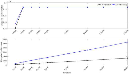
Objective function value (profit) and computation time of Case 1 as function of the number of iterations
Objective function value (profit) and computation time of Case 1 as function of the number of iterations
As it can be seen from Figure 1, the genetic algorithms converge after around 20k iterations to a stable solution for both population sizes. The convergence is faster with a larger population size. Moreover, the computation time is an increasing linear function of the number of iterations with a larger slope for the larger population size case. The solution is provided in Table 1. The only excluded port from the service is P15: Khor Fakkan. The optimal sailing speed of 24 kt witnesses the choice of a high speed level to have the maximum positive impact on the collected revenues.
Heuristic solution of the 17-port cases
| Cases | Z (US$ per cycle) | Selected speed (kt) | NV | Selected route |
|---|---|---|---|---|
| Case 1 | 128 630 583 | 24 for all arcs | 9 | P1, P5, P4, P17, P6, P7, P16, P8, P9, P14, P10, P13, P12, P11, P2, P3, P1 |
| Case 2 | 95 405 651 | 24 for all arcs | 9 | P1, P5, P4, P17, P6, P7, P16, P8, P9, P14, P10, P13, P12, P11, P2, P3, P1 |
| Case 3 | 134 000 821 | 18.4, 22, 24, 22.2, 22, 24, 23.6, 24, 24, 22.6, 24, 21.6, 20.2, 18.2, 16, 20, 20 | 11 | P1, P5, P4, P17, P6, P7, P16, P15, P8, P14, P10, P13, P12, P11, P9, P2, P3, P1 |
| Case 4 | 24 956 791 | 21, 21.6, 21.6, 21.8, 21, 22.2, 21.2, 22, 22, 22.4, 22.4, 21.6, 20.2, 18.2, 17.2, 18.4, 20.6 | 11 | P1, P5, P4, P17, P6, P7, P16, P15, P8, P14, P10, P13, P12, P11, P9, P2, P3, P1 |
| Case 5 | 62 338 724 | 24 for all arcs | 9 | P1, P5, P4, P17, P6, P7, P16, P8, P9, P14, P10, P13, P12, P11, P2, P3, P1 |
4.3 Effect of the bunker price combined with the demand sensitivity
To assess the effect of the bunker price and of the demand sensitivity on the obtained solution, the problem has been solved using the same input data as for Case 1, except the bunker price and the demand sensitivity to the sailing speed. The following combinations have been tested:
Case 2: , and
Case 3: , and
Case 4: , and
The results are shown in Table 1.
The obtained results confirm that the proposed algorithm converges towards a heuristic solution, and that the convergence is faster, in general, with the smallest population size, i.e. 39 individuals. Moreover, the convergence happens generally after 100k iterations. Moreover, the computation time is a linear function of the number of iterations and that it is longer for the case with larger population size. The difference increases with the number of iterations.
Table 1 shows clearly the effect of the bunker price on the heuristic solution. When the bunker price increases, as in Case 2, the heuristic profit decreases, while in this case, the corresponding solution, including the selected ports and the vessel sailing speed do not change. This is mainly due to the demand sensitivity to the sailing speed. However, when the bunker price increases further, as in Case 3 and Case 4, the sailing speeds decrease further. This decrease is not the same for all arcs and this is due to the demand value between the different ports. In Case 3, however, the profit increases slightly compared to Case 1 due to the fact that in this solution, P15 is included. The average sailing speed of Case 3 is 21.57 kt while the average sailing speed of Case 4 is 20.90 kt. The difference is due to bunker price. However, the number of vessels of both cases is 11.
It can be noted that, when the obtained heuristic best speed is the same for all legs, the convergence of the algorithm seems to be faster.
4.4 Impact of the vessel size
To assess the impact of the vessel size on the results, we consider for the same service described earlier, a new vessel size (Woo, 2012):
10000 TEU out of which 10% is dedicated to reefer containers with: PSE = 74000 kW, PSAux = 12000 kW, ELE = 0.9, ELAux =0.5, SFOCE = 307 g/kWh, SFOCAux = 221 g/kWh, Cv = 74658 US$/day.
All the other parameters detailed in Section 4.1 remain unchanged. However, the standard revenues generated and the reefer demand considered in Section 4.1 were multiplied by a factor of 0.71, to account for the smaller vessel capacity. This case is called Case 5.
The results confirmed that the algorithm performance is similar to Case 1 in terms of convergence and computation time. It can also be noted that the heuristic profit obtained is almost half the profit collected by Case 1. This is due to the vessel size and to the demand that is smaller in this case than in Case 1.
4.5 Large size cases
In addition to the previous results, we discuss here a larger size problem, in which 25 ports are included: P1: Tokyo, P2: Busan, P3: Dalian, P4: Shanghai, P5: Ningbo, P6: Xiamen, P7: Shenzhen, P8: Vung Tau, P9: Port Klang, P10: Tanjung Pelepas, P11: Colombo, P12: Mundra, P13: Karachi, P14: Jabel Ali, P15: Jeddah, P16: Piraeus, P17: Gioia Tauro, P18: Malta, P19: Algeciras, P20: Le Havre, P21: Southampton, P22: Felixstowe, P23: Rotterdam, P24: Bremerhaven, P25: Hamburg.
We considered the same vessel size used in Section 4.1, i.e. an average nominal capacity of 14,000 TEU out of which 10% of reefer slots. The sailing distances between the ports have been obtained from Sea Distance (2018). The port time values, for all the ports were assumed to be equal to one day RTi = 1 day.
The standard times between the ports, , have been calculated based on a standard direct sailing speed of 16 knots in addition to half the port times. The total standard revenues between the ports have been obtained from World Freight Rate (2018). The expected standard reefer quantities, , and the corresponding freight rates, , are available from the authors upon request. It is worth noting that the reefer freight rates have been obtained by multiplying the freight rates obtained from World Freight Rate (2018) by 2. Moreover, the heuristic parameters, i.e. the population size, the number of iterations and the sailing speed discretization step are the same as the ones described in Section 4.1. This case is referred to as Case 6.
The results are shown in Table 2. The results show that the only two excluded ports from the service are P16: Piraeus and P18: Malta. The justification may be related to their revenues versus the additional sailing and port times spent to call at these ports. It is obvious that the computation time is slightly higher in this large size instance compared to the previous cases. Moreover, the convergence seems also slower than in the smaller cases.
Heuristic solution for the large size cases
| Cases | Z | V | NV | Selected route |
|---|---|---|---|---|
| Case 6 | 219 698 600 | 24 for all arcs | 16 | P1, P3, P2, P4, P5, P6, P7, P8, P19, P20, P22, P23, P24, P25, P21, P17, P15, P13, P12, P11, P9, P10, P14, P1 |
| Case 7 | 155 234 202 | 10, 16.8, 24, 24, 24, 24, 24, 24, 24, 24, 24, 24, 24, 24, 24, 24, 24, 24, 24, 24, 13.8, 10.8 | 12 | P1, P3, P2, P4, P5, P6, P7, P8, P20, P22, P24, P25, P23, P21, P19, P17, P15, P13, P12, P11, P9, P10, P1 |
| Case 8 | 120 936 968 | 12.4, 24, 24, 24, 24, 24, 24, 24, 24, 24, 24, 24, 24, 24, 24, 24, 24, 24, 24, 24, 23.2, 16.2 | 11 | P1, P2, P3, P4, P5, P6, P7, P8, P19, P20, P22, P23, P24, P25, P21, P17, P15, P13, P12, P11, P9, P10, P1 |
| Case 9 | 230 838 366 | 20.8, 24, 24, 24, 24, 24, 24, 24, 24, 24, 24, 24, 24, 24, 24, 24, 24, 22, 22, 24, 15.6, 21, 19.2, 20, 16 | 12 | P1, P2, P3, P4, P5, P6, P7, P8, P9, P12, P13, P14, P21, P22, P24, P25, P23, P20, P19, P17, P18, P16, P15, P11, P10, P1 |
| Case 10 | 93 878 643 | 18, 19.6, 20.4, 21, 22.2, 22.2, 23.6, 23.2, 22.4, 23.8, 22.4, 22.4, 23.6, 22.8, 21.6, 21, 20, 19.4, 18, 16.4, 17.6, 17.2, 17.4 | 12 | P1, P2, P3, P4, P5, P6, P7, P8, P9, P12, P13, P15, P21, P23, P25, P24, P22, P20, P19, P17, P16, P11, P10, P1 |
4.6 Impact of fuel price and demand sensitivity on large size cases
In addition, the same three fuel price and demand sensitivity scenarios defined in Section 4.3 have been also used for the large size problem with 25 ports in addition to forth scenario (Case 8). All the model parameters defined in Section 4.5 have been used except the fuel price and the demand sensitivity that are given hereafter which results in four new cases referred to as:
Case 7: , and
Case 8: , and
Case 9: , and
Case 10: , and
The results are shown in Table 2.
The results confirm that it takes longer time for the algorithm to converge with the larger size problems, compared to the smaller size ones. However, the larger population size seems to converge faster than the case with smaller population size. The main findings would be the following:
Comparing Case 6 with Case 7, one can see that when the bunker price increases the sailing speeds decrease, the number of included ports decrease as well as the generated profit. At the same time, the needed number of vessels decreased because of the drop of ports from the service.
Comparing Case 7 with Case 8, one can see that the number of selected ports decreases further due to the increase of the bunker price. In addition, the required number of vessels decreases to 11 as well as the generated profit. However the average sailing speed in Case 8 is 23.08 kt while for Case 7 it is 21.97 kt. Therefore, although the bunker price increased in Case 8, due to the decrease of the number of vessels, the sailing speed increased to compensate and not to affect the collected revenues.
Comparing Case 8 with Case 9, that have the same bunker price but different demand sensitivities, Case 9 being less sensitive to the transit time, one can notice that Case 9 generates much more profit. Moreover, the selected number of ports increased in Case 9 when the demand sensitivity decreased. In addition, the average sailing speed in Case 8 is 23.08 kt, while it is equal to 22.58 kt in Case 9, while the number of vessels in Case 9 is one more than for Case 8. This is natural since when the demand sensitivity decreases, the sailing speed decreases to reduce the bunker cost, while the number of vessels increases to compensate.
Comparing Case 9 and Case 10 confirms clearly the impact of the bunker price on the profit, the sailing speed and the included ports in the service.
5. Conclusion
This paper proposes a mathematical model for liner shipping service. The model is based on a multi-vessel TSP with profit formulation and on an accurate estimation of the total liner service cost. The model considers an important aspect of the market in which the transport demand, and therefore, the corresponding revenue is sensitive to the sailing speed. Moreover, a heuristic optimization procedure based on a genetic algorithm is proposed. A numerical application is conducted based on a liner service that was operated in 2017 by COSCO between Asia and Europe. Two other cases with different vessel size or different number of ports have also been analysed. We implemented the heuristic in Matlab R2015 and obtained the heuristic solution for this basic case as well as for some cases in which the effect of the bunker price and the demand sensitivity have been investigated. The results show that the heuristic solutions of the model are sensitive to the bunker price as well as to the sensitivity level of the transport demand. The proposed model and the solution approach can provide container shipping companies with a simple decision-making tool to determine the best route for their liner services, find the corresponding optimal profits and, consequently, design their networks. Considering the capacity limitations in the model can be an avenue for future research.