
The authors examine the contemporaneous and causal association between tweet features (bullishness, message volume and investor agreement) and market features (stock returns, trading volume and volatility) using 140 South African companies and a dataset of firm-level Twitter messages extracted from Bloomberg for the period 1 January 2015 to 31 March 2020.
Panel regressions with ticker fixed-effects are used to examine the contemporaneous link between tweet features and market features. To examine the link between the magnitude of tweet features and stock market features, the study uses quantile regression.
No monotonic relationship is found between the magnitude of tweet features and the magnitude of market features. The authors find no evidence that past values of tweet features can predict forthcoming stock returns using daily data while weekly and monthly data shows that past values of tweet features contain useful information that can predict the future values of stock returns.
The study is among the earlier to examine the association between textual sentiment from social media and market features in a South African context. The exploration of the relationship across the distribution of the stock market features gives new insights away from the traditional approaches which investigate the relationship at the mean.
1. Introduction
While classical finance postulates that investors are rational and build their portfolios using mean-variance optimisation, behavioural finance suggests that investors are normal individuals who build their portfolios using the behavioural portfolio theory (Statman, 2019). Behavioural finance proponents have challenged the theoretical underpinnings of the efficient markets hypothesis (EMH) as well as the accompanying empirical evidence by arguing that investors are not perfectly rational and therefore capital markets are not perfectly efficient. By trying to give a more plausible explanation of asset pricing, behavioural finance incorporates concepts from the diverse fields of finance, psychology and sociology (Shiller, 2003). One aspect of behavioural finance that has received extensive research in recent times is the role of investor sentiment in financial markets. Black (1986) suggests that irrational investors, also called noise traders, are known for not trading on fundamental information but are instead driven by sentiment. Several studies across the developed world, as well as developing countries, have confirmed the importance of investor sentiment in financial markets.
While most studies have used survey-based measures of investor sentiment, the notion of textual sentiment from social media is an emerging form of investor sentiment which is text-based and portrays the level of positivity and negativity in texts from social media platforms like blogs and microblogs (Li et al., 2018). This form of investor sentiment has been driven by the proliferation of algorithms that deduct sentiment from text and the parallel increase in the interactions among investors using microblogs, social media sites, discussion forums and internet message boards. Many individual traders are abandoning traditional news platforms for social media platforms as the former allows users to express their opinions in addition to obtaining information (Kearney and Liu, 2014). Twitter and StockTwits have emerged as some of the most used online microblogs that finance and computer science researchers are using to extract textual sentiment (Li et al., 2018).
Using data from 140 listed shares on the main board of the Johannesburg Stock Exchange, we investigate whether tweet features (bullishness, message agreement and message volume) are associated with market features (stock returns, trading volume and volatility). Twitter and StockTwits platforms have been chosen for this study ahead of other microblogs because they are some of the most used by the investing community. These platforms allow participants to tap into the “wisdom of crowds”, where the sum of information emanating from multiple novice investors is presumed to predict outcomes more accurately than experts (Bartov et al., 2018). Also, the short format of the platforms (up to 280 characters) and ease of information search (for example the use of cashtags, which are stock ticker symbols prefixed with a dollar sign), make them the ideal media to share information promptly and therefore relevant for a study of this nature. One of the pioneering studies that examined the role of sentiment extracted from tweets in the financial markets (Bollen et al., 2011) led to the formation of the world's first Twitter-based hedge fund (Thompson, 2011). A study of this nature, therefore, helps to establish if investment strategies based on social media are feasible in an emerging economy like South Africa. Several studies done on the effect of investor sentiment on stock market features in South Africa have mainly used low-frequency data (e.g Solanki and Seetharam, 2018). We depart from this approach and adopt high-frequency data sampled at the daily level to reflect the spontaneity of noise traders. The choice of South Africa is premised on its globally recognised standard of regulation as well as its often classification as either emerging or developed (Seetharam, 2021). This has consequences on the dynamics of financial markets. For example, China and South Korea are emerging markets whose stock markets are dominated by individual investors while the Johannesburg Stock Exchange mirrors developed stock exchanges as it is dominated by institutional investors. Specifically, we seek to address the three objectives below:
Determine if firm-level tweet features are contemporaneously associated with stock market features;
Determine if the magnitude of tweet features is monotonically related to the magnitude of stock market features;
Determine if past values of tweet features contain useful information that could be used to predict future values of stock returns.
In this study we use the following stock market features; stock returns, trading volume and return volatility. Though studies have been done that examine the linkages between the social media features used in this study and stock market features (such as Sprenger et al., 2014), our study adds to the literature on this topic in several ways. Unlike other studies that are restricted to associations at the mean (such as Allen et al., 2019; Sprenger et al., 2014), this study utilises the quantile regression approach to capture the linkage between tweet features and market features across the conditional distribution of the dependent variable. This methodological enhancement, therefore, offers new insights that enrich the extant literature on textual sentiment in the stock market, especially in the context of South Africa. Also, our study uses a novel database of Twitter sentiment from Bloomberg that has been used in other countries like Zimbabwe (Nyakurukwa and Seetharam, 2021) and the United States of America (Gu and Kurov, 2020) but has not been used in a South African context to the best of our knowledge. Bloomberg Inc has become an important platform for capital market analysts as statistics show that more than 320,000 of the world's most influential decision-makers are part of the community [1].
The findings from the study show a general significant contemporaneous relationship between tweet features and stock market features. The analysis of the quantile relationships between tweet features and stock market features suggests that the relationship between the features is heterogeneous across the distribution of the returns with tweet features particularly strong during states of extreme returns. The lead-lag relationship between tweet features and stock returns is frequency-dependent, with no relationship found at the daily interval while bidirectional causality is established at the weekly and monthly intervals.
2. Literature review
2.1 Theoretical framework
Long considered the cornerstone of modern financial theory, the EMH states that capital markets are informationally efficient as they instantaneously assimilate all available information (Fama, 1970). According to this hypothesis, the arrival of new information in capital markets leads to the prompt correction of the prices of stocks to their “correct values” (Malkiel, 2003). The EMH is closely related to the notion of a stochastic process which postulates that asset prices do not have a memory and that future price changes represent random deviations from prior prices (Malkiel, 2003). By definition, the coming of new information is presumed to be a chance event and as such, subsequent prices are also anticipated to be erratic and unpredictable. This characteristic of share prices, in principle, means that it is not feasible to attain returns that exceed risk-adjusted market returns.
In the 1980s, many economists started questioning the EMH by arguing that stock prices are somewhat predictable. These researchers emphasised the importance of psychological and behavioural factors in asset pricing. Studies done by behavioural finance economists have largely shown that stock prices are predictable and that it is possible to earn a riskless profit based on historic prices as well as the use of certain fundamental valuation metrics (Malkiel, 2003). While finance discourse has been dominated by advocates of the EMH and behavioural finance paradigms, there is an emerging crop of scholars who do not subscribe to the notion of fully efficient markets, nor to markets that can be explained solely by behavioural theories. Lo's (2004) Adaptive Market Hypothesis (AMH) attempts to reconcile the two ideologies by using explanations from evolutionary sciences. The AMH views asset prices in financial markets as reflecting a combination of environmental factors as well as the nature and number of participants (species) in the environment. The diversity of the market participants (such as naïve investors, smart investors, market makers) makes financial markets' efficiency context-specific.
2.2 Empirical literature and hypotheses development
Several studies have been done on the contemporaneous associations between textual sentiment and stock market features like stock returns, volatility and trading volume. Sprenger et al. (2014) analyse 250,000 stock-related tweets to determine if sentiment from tweets can impact stock returns, volatility and trading volume. The authors report that bullishness, message volume and message disagreement are positively and significantly related to the stock market features of stock returns, volatility and trading volume. Li et al. (2018) assemble more than one million tweets for 100 companies listed on the S&P500. Using 15-min-interval intraday granularity which is more relevant for real-time microblogs like Twitter, the study shows that the message features used had a positive effect on stock returns, trading volume and volatility. Consistent with Antweiler and Frank (2004), Li et al. (2018) report that disagreement induces trading. This leads to our first hypothesis:
Firm-level tweet features (bullishness, message volume and investor disagreement) are positively and contemporaneously associated with market features (stock returns, trading volume and volatility).
Although various studies have been done to establish the association between sentiment from microblogs and stock market features, there is still widespread debate on when textual sentiment matters most for investors. Studies that have been done to investigate when investor sentiment matters have largely produced mixed results. While Shleifer and Vishny (1997) show that the impact of sentiment on share returns should be symmetric, a complex relationship is likely to arise because of the variations in shorting expenses from different market conditions. Stambaugh et al. (2012) posit that the differences in shorting costs and therefore shorting impediments in different market conditions should make overpricing prevail over underpricing. Smart investors are therefore more likely to enter capital markets following bullish rather than bearish market conditions and hence predictability should be more pronounced during good market conditions (Lemmon and Portniaguina, 2006).
Contrary to the above-mentioned phenomenon, Prospect Theory suggests that the expected utility theorem does not adequately capture human behaviour in the face of gains or losses (Kahneman and Tversky, 1979). According to Prospect Theory, individual investors are susceptible to significant pain from a loss compared to excitement from a gain of comparable magnitude (Kahneman and Tversky, 1979). This proposition asserts that the behaviour of investors varies significantly, contingent upon the state of the capital markets and whether they are characterised by periods of anxiety and fear or by prosperity and tranquillity. Related to this, studies have also shown that investors are more likely to be irrational during periods of anxiety. All this points to a more pronounced prediction of stock market features during bad times compared to good times. Ma et al. (2018) report results that are consistent with this phenomenon, using sentiment extracted from macroeconomic variables through principal component analysis. The study uses a quantile regression approach and concludes that the prediction of stock returns using investor sentiment is more pronounced at lower and middle return quantiles . However, at upper quantiles , the forecasting power of sentiment is lost and the regression coefficients become anomalous. Hillert et al. (2018) utilise disagreement among journalists as a proxy for investor disagreement. The results from the study show that the disagreement metric constructed to measure journalist disagreement is inversely associated with market returns and that the connection is more pronounced during bear periods. The above two phenomena show that it is likely that the magnitude of the tweet features is not monotonically related to the magnitude of stock returns leading to our second hypothesis:
The magnitude of firm-level tweet features is not monotonically related to the magnitude of stock returns.
While it is important to know the contemporaneous association between tweet features and stock market features, it is more important to know whether past values of tweet features contain useful information that could be used to predict future returns. One of the earliest documented studies to examine the information content of textual sentiment extracted from Twitter was done by Bollen et al. (2011). Granger non-causality and a Self-Organising Fuzzy Neural Network were employed to test the forecasting power of specific public mood states on the Dow Jones closing prices. The study concluded that public mood states can predict the changes in the closing prices of the Dow Jones. Because western social media platforms are banned in China, Xu et al. (2017) use an indigenous Chinese Twitter-like social media platform, Sina Weibo, to extract textual sentiment. On the lead-lag relationships, stock returns are found to cause Weibo sentiments than the other way round. Message disagreement is also found to contain useful information associated with trading volume. This is consistent with the “no-trade theorem” which states that disagreement induces no trading as it necessitates the review of prices and opinions (Milgrom and Stokey, 1982). This leads us to our third hypothesis:
Past values of tweet features (bullishness, investor disagreement and message volume) contain useful information that could be used to predict future stock returns.
3. Methodology
3.1 Data
The study examines whether firm-level tweet features can explain stock market features. To investigate the aforementioned, the study utilises firm-level data for all FTSE/JSE All Share Index (JALSH) constituent firms for the period 1 January 2015 to 31 March 2020. Firm-level daily data on tweet features, closing prices, low prices, high prices, trading volume and market capitalisation are extracted from the Bloomberg terminal. Returns are adjusted for corporate actions and/or dividends where applicable. Only the current JALSH constituent companies are included in the study as they are the only companies for which tweet features data are available on the Bloomberg terminal. This means companies that were part of the JALSH during the sample period but exited the index before 31 March 2020 are excluded from the analysis. This leads to a dataset with 140 firms, 1,247 trading days and 197,026 firm-days.
The sample period is limited to the period after 1 January 2015 as Bloomberg only started incorporating tweet features data for JALSH firms on its platforms in 2015. Since only daily tweet features' data are available from Bloomberg, the study primarily uses daily granularity analysis. Bloomberg aggregates the tweets of a specific listed company at the end of the day where aggregation leads to aggregated tweets containing positive, negative and neutral sentiment. This means that the tweets of a particular share are aggregated at the end of the day to create a single observation for that day.
3.2 Variables
This section defines the variables used in this study as well as justification for their inclusion in the study:
3.2.1 Tweet features
Following Sprenger et al. (2014), three tweet features are used as the explanatory variables: namely; bullishness (), message volume () and message agreement (). The process of calculating the bullishness index (called average sentiment in the Bloomberg terminal [2]) used by Bloomberg Inc. is explained in detail in Appendix 2.
Bullishness ranges from −1, the most negative sentiment to +1, the most positive sentiment. This means that a bullishness score of 0 denotes neutral sentiment. Bloomberg provides the daily total number of tweets for each firm aggregated at the end of the day. Message volume () in this study is calculated as the natural logarithm of the aggregate tweets for stock at time interval . The message agreement index () reflects the extent of the consensus among microbloggers on the prospects of each stock at time-variable . Following Antweiler and Frank (2004), the following is used to measure message agreement:
where indicate the number of messages which are respectively categorised as positive and negative. If all the messages at a given time are equally distributed between positive and negative, it means that there is absolute agreement among microbloggers and therefore the value of will be equivalent to 1. In a situation where all messages are either positive or negative, then it means microbloggers are in total disagreement and the agreement index will therefore be 0. Thus, the closer the agreement index is to 0, the greater the disagreement among stock microbloggers while a value close to 1 indicates greater agreement. The major advantage of the above agreement metric is that it directly measures the dispersion of investor opinions compared to alternative metrics which rely on indirect measures like volatility and analyst forecast dispersion. Additionally, the agreement measure is computed at the daily level compared to alternative metrics which are usually measured at lower monthly and quarterly frequencies (Diether et al., 2002).
The challenge with the agreement index above is that there are companies that go for a considerable time without being mentioned on Twitter and StockTwits forums, leading to missing values for the tweet features. Consistent with Sprenger et al. (2014), this study assigns a value of zero to bullishness and message volume for all “quiet” periods. Imputing zero values to the bullishness scores of companies that are not mentioned on the Twitter and StockTwits platforms on any day is done on the presumption that when investors do not mention a specific counter, this means that they are neutral on the prospects of the counter. To compute the agreement index, “zero” values are assigned to and respectively in periods when either one or all of them are “quiet”. The agreement index is then computed accordingly. Another potential problem with the agreement index described above is that since it is computed using the raw number of messages posted, it might be biased for companies that have very low levels of messages posted about them on Twitter, especially at the daily interval. This can be seen from the distribution of the number of messages posted for the whole sample as the minimum number of messages posted is 1 at the daily frequency. This possible challenge is ameliorated by using weekly and monthly data in the further analysis done as the minimum number of messages posted are 2,991 and 6,027 respectively.
3.2.2 Market features
Three stock market features are used in the study, namely; raw returns (), Volatility () and Trading Volume (). Raw returns () for stock at time interval are defined as:
where stands for the closing price at time interval and stands for the closing price at time interval . For holidays when there is no trading on the JSE, missing values are imputed using the average of the closing price a day before and a day after the missing value day. Since holidays represent a small percentage (less than 2%) of the observations, this is not expected to have a significant effect on the findings.
This study uses a volatility estimation model that captures drops and recoveries of financial markets daily instead of the classical close-to-close volatility models. Volatility () is estimated using intraday price highs and lows in line with the PARK volatility measure (Parkinson, 1980). The PARK estimator's accuracy instinctively emanates from the idea that the intraday price range gives more information regarding future volatility than two arbitrary closing-price points in the series. Supposing that the stock price follows a simple Brownian model without a constant term, the PARK statistic is calculated as follows:
where stand for the daily highs and lows of a stock price at time . PARK volatility has also been used in scholarly articles examining the role of textual sentiment in capital markets (such as Sprenger et al., 2014; Li et al., 2018). Trading volume is estimated as the natural logarithm of the traded volume of stock at time .
3.3 Econometric model
3.3.1 Contemporaneous relationship between tweet features and stock market features
Panel regressions with ticker fixed-effects are used to examine the contemporaneous link between tweet features and market features as shown in Equation (4). This model follows that of Sprenger et al. (2014) where all the tweet features are used as covariates and the market index is included as a control variable as shown below:
where
represents the three market features (firm-level stock returns, volatility and trading volume) of firm at time ;
is the bullishness score of firm at time interval ;
represents message volume of firm at time interval ;
represents message agreement for firm at time interval ;
is the market return calculated as the natural logarithm of the closing value of the JALSH index at time divided by the value at time ;
is an error term that is clustered by ticker;
is the unknown intercept for every company
3.3.2 Examining if the magnitude of tweet features is monotonically related to the magnitude of market features
To examine the link between the magnitude of tweet features and stock market features, the study uses quantile regression. This type of model was first proposed by Koenker and Bassett (1978) and allows the researcher to drop the assumption that variables operate the same at the lower and upper tails as at the mean. It, therefore, allows understanding the relationships between variables outside of the mean. While some studies have used the sample splitting procedure to examine the magnitude and significance of investor sentiment at different market conditions, Koenker (2004) argues that the procedure leads to severe sample selection complications. Quantile regression necessitates the approximation of conditional quantiles of the regressand given a range of predictor variables without splitting the sample (Koenker and Bassett, 1978). The quantile regression estimator also permits the effect of the explanatory variable to fluctuate across quantiles of the dependent variable.
Some of the documented advantages of quantile regression estimators include the fact that they are robust to outliers and they deal with non-linearity without presuming a specific form of the model (Koenker and Bassett, 1978). Using quantile regression, the conditional quantile function of at quantile given explanatory variable is defined as follows:
where stands for the distribution of errors and and are the parameters. The coefficients of the conditional quantile regression are approximated as follows:
where T indicates the sample size and is the check function defined as if and otherwise. Since quantile regression is an extension of linear regression, this study uses Equation (4) as the baseline equation for the quantile regression model specification as follows:
where is the quantile in the conditional distribution of the regressand. Equation (7) is the quantile regression model which is estimated to establish whether the magnitude of sentiment is linked to the magnitude of stock return. Five quantile intervals representing the different market conditions as shown by the firm-level stock returns are used as follows: where represent bad market conditions, represents normal market conditions and represent good market conditions.
3.3.3 Examining if past values of tweet features contain useful information that could be used to predict future values of returns
To examine whether past values of tweet features contain useful information that could be used to predict future values of stock returns, the study utilises Granger non-causality tests (Granger, 1969). According to Granger (1969), a causal relationship is inferred when the lagged values of a variable have explanatory power in a regression of a variable on lagged values of . To test whether (representing the tweets features) Granger-causes (representing stock returns), the Wald statistic for heterogenous panels proposed by Dumitrescu and Hurlin (2012) is used. The test statistic Dumitrescu and Hurlin (2012) propose is a simple average of individual Wald statistics obtained from testing the null hypothesis for every cross-sectional unit in the panel. The test is based on the stationary fixed-effects panel model:
where and are the tweets features and the stock returns respectively. The optimal lag length is selected using the lag length that minimises the Akaike Information Criterion (AIC), Bayesian Information Criterion (BIC) and Hannan-Quinn Information Criterion (HQIC). The “homogenous non-causality” null hypothesis of the Dumitrescu and Hurlin (2012) statistic is given below:
where it is assumed that there is no causal relationship under the null hypothesis for all N while causal relationships are assumed under the alternative hypothesis where . is assumed to be unknown and will comply with the condition .
The predictive power of tweet features on stock returns is further investigated using weekly and monthly data. Various studies that have examined the information content of investor sentiment in a South African context have mostly used monthly survey data and the majority have confirmed the information content of investor sentiment in predicting future values of stock returns (such as Dalika and Seetharam, 2015). To find the weekly and monthly scores for message volume and investor agreement, the daily tweet features are aggregated at the end of every week and month respectively. The weekly and monthly bullishness scores are then calculated in line with Antweiler and Frank (2004) using the following formula:
where is the bullishness score for firm at time , where time is at weekly and monthly intervals. The weekly and monthly returns are calculated as the natural logarithm of the stock price at () divided by the stock price at (). Granger non-causality is estimated using a simple F-test where the null hypothesis is that the tweet features do not Granger cause stock returns and vice-versa.
3.4 Robustness checks
To mitigate methodological choices from driving the results, some econometric models above are re-estimated using a multitude of alternative specifications which are outlined in this section. The model to test the contemporaneous association between tweet features and stock market features using ticker fixed effects is re-estimated using random effects. Testing the linkages between the magnitude of tweet features and stock market features using five quantiles in a quantile regression model is re-estimated using . Finally, the information content of tweet features in predicting stock returns is further assessed using lead-lag Fama-Macbeth style regressions. In estimating the Fama-Macbeth regression, the two pass-regression process firstly estimates the cross-sectional regressions of the firm-level market features and stock returns for each day. This is followed by estimating the averages of the daily coefficients and reporting the standard errors of the estimates. Heteroskedasticity-consistent standard errors are reported to deal with heteroskedasticity and autocorrelation concerns of dealing with panel data. Like previous studies, the study controls for size using the natural logarithm of the firms' market capitalisation. One and two-day lags of tweet features are regressed on stock returns separately and vice-versa to establish the direction of prediction. Lagged tweet features have information content if their coefficients are statistically significant at the 5% level.
4. Results and discussion
4.1 Descriptive statistics
Table 1 shows the summary statistics of the market and microblog features for the daily granular data used in the study. The panel data includes observations of the tweet and market features for a period of 1,247 trading days from 2015 to 2020, together making a total of 197,026 firm-days.
Summary statistics of the variables
| Statistic | N | Mean | SD | Med | Min | Max |
|---|---|---|---|---|---|---|
| Tweet features | ||||||
| Bullishness | 197,026 | 0.0020 | 0.1035 | 0.0000 | −0.0069 | 0.9978 |
| Messages | 197,026 | 0.4133 | 0.9295 | 0.0000 | 0.0000 | 7.8860 |
| Agreement | 197,026 | 0.0212 | 0.0605 | 0.0000 | 0.0000 | 0.8549 |
| Market features | ||||||
| Stock returns | 197,026 | −0.0001 | 0.0232 | 0.0000 | −0.9525 | 0.4964 |
| Trading volume | 197,026 | 13.0393 | 1.8832 | 13.34898 | 0.0000 | 28.7688 |
| Volatility | 197,026 | 26.4899 | 8.1698 | 26.2757 | 6.8702 | 56.5512 |
| Size | 197,026 | 23.8417 | 1.4584 | 23.6327 | 17.4128 | 28.7688 |
| Market return | 197,026 | 0.0001 | 0.0093 | 0.00046 | −0.03621 | 0.03649 |
Note(s): N shows the total number of observations, St.Dev shows the standard deviation of the variables while Med, Min and Max represent the median, minimum value as well as maximum value of the variables respectively
As shown in Table 1, bullishness ranges from a minimum value of −0.0069 to a maximum value of 0.9978 showing that textual sentiment as measured by bullishness fluctuates across the polar estimates. On average, bullishness is +0.002, which is positive but close to 0 showing that the sentiment of investors was only slightly positive and therefore near neutral. The distribution of the number of firm-level tweets by day of the week is visually depicted in Figure 1.
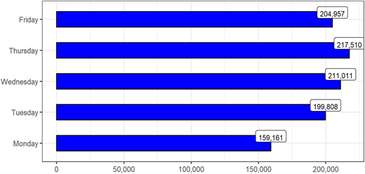
The total number of times the sampled companies were mentioned on the Twitter and StockTwits platforms is 992,447. The distribution of the tweets by day of the week shows that the volume of stock-related messages is low at the beginning of the week and gradually increases until it peaks on Thursdays and thereafter subsides.
4.2 Contemporaneous relationship between tweet features and market features
This section presents the results on the contemporaneous associations between the tweet features and market features to establish whether tweets can contemporaneously explain the cross-section of market features for JALSH constituent companies. The results from the contemporaneous OLS estimations with firm-fixed effects are shown in Table 2.
Contemporaneous OLS regressions with firm fixed effects
| Dependent variable | |||
|---|---|---|---|
| Return (1) | Volatility (2) | Trading volume (2) | |
| Bullishness | 0.004*** (0.001) | 1.086*** (0.046) | −0.000 (0.026) |
| Agreement | −0.004*** (0.001) | −1.647*** (0.084) | 0.209*** (0.047) |
| Messages | 0.0001 (0.0001) | −0.208*** (0.008) | 0.083*** (0.004) |
| Market return | 0.615*** (0.006) | 0.450 (0.467) | −0.867*** (0.262) |
| Constant | −0.001 (0.003) | 0.001 (0.003) | −0.002 (0.003) |
| Observations | 180,724 | 180,887 | 180,881 |
| 0.062 | 0.011 | 0.002 | |
| 0.061 | 0.010 | 0.002 | |
| F statistic | 2.997.6*** (df = 4) | 500.5*** (df = 4) | 108.4*** (df = 4) |
Note(s): The table reports the regression coefficients of the models estimated, standard errors are reported (in brackets), *p < 0.1; **p < 0.05; ***p < 0.01
In Table 2, Models 1, 2 and 3 show the regressions of returns, volatility and trading volume on the tweet features respectively. The findings reveal that bullishness is directly and significantly associated with stock returns. Quality and content seem to be more important than quantity since bullishness is related to returns more strongly than message volume. The relationship between the agreement index and stock returns is negative and statistically significant at 1% showing that disagreement among microbloggers is associated with higher stock returns. This is in line with previous studies that report a negative and significant relationship between investor agreement using texts extracted from Yahoo! Finance (Antweiler and Frank, 2004) and Twitter (Li et al., 2018; Sprenger et al., 2014). The relationship between message volume and stock returns, though positive , is not significant at any of the conventional levels. This is consistent with Sprenger et al. (2014) who found no significant relationship between the natural logarithm of the volume of firm-level tweets and firm-level returns. These results are however contrary to the findings of Antweiler and Frank (2004) and Li et al. (2018) who found a positive and significant relationship between message volume and stock returns.
Table 2 also shows that volatility is significantly associated with all the tweet features. Firstly, volatility is positively and significantly associated with bullishness . This is consistent with previous studies which report a positive and significant relationship between volatility and bullishness (Kim and Kim, 2014; Sprenger et al., 2014). As expected, volatility is negatively and significantly associated with agreement This means that increased dispersion of investor opinion on stock microblogs is associated with higher volatility. Volatility is also negatively and significantly associated with the volume of firm-level tweets . This is contrary to the majority of previous studies which largely report a significant and direct link between message volume and volatility (Antweiler and Frank, 2004; Sprenger et al., 2014).
On the contemporaneous relationship between trading volume and the tweet features, in line with Li et al. (2018), Table 2 shows no statistically significant relationship between bullishness and trading volume. On the other hand, the link between message volume and trading volume is positive and statistically significant at the 1% level . Since the values for message volume and trading volume are both log transformed, they can be interpreted as elasticities. This means that a 1% increase in message volume is associated with a more than 8% increase in trading voume. This result is almost quantitively and qualitatively similar to Sprenger et al. (2014) who report a 1% increase in message volume being associated with a 10% increase in trading volume. The positive relationship between message volume and trading volume means that microblog users on Twitter post messages of companies that are traded more heavily (Sprenger et al., 2014). Contrary to previous studies (such as Antweiler and Frank, 2004; Li et al., 2018), the relationship between the agreement index and trading volume shown in Table 2 is positive. This is in line with literature that recognises that information differences need to interact with some other forms of heterogeneity, like heterogeneous beliefs, to generate trading (Sprenger et al., 2014). However, the extent to which how much each source of disagreement matters for trading is an open question. The results in Table 2 are qualitatively similar to the results using an OLS model with random effects reported in Table A1 in Appendix.
Random effects estimation
| Dependent variable | |||
|---|---|---|---|
| Return (1) | Volatility (2) | Trading volume (2) | |
| Bullishness | 0.004*** (0.001) | 1.086*** (0.046) | −0.0002 (0.026) |
| Agreement | −0.004*** (0.001) | −1.647*** (0.008) | 0.211*** (0.004) |
| Messages | 0.0001 (0.0001) | −0.208*** (0.008) | 0.084*** (0.004) |
| Market return | 0.615*** (0.006) | 0.450 (0.467) | −0.867*** (0.262) |
| Constant | −0.0003*** (0.0001) | 26.606*** (0.587) | 13.014*** (0.119) |
| Observations | 180,724 | 180,887 | 180,881 |
| 0.062 | 0.011 | 0.004 | |
| Adjusted R2 | 0.062 | 0.010 | 0.004 |
| F-statistic | 11,993.42*** | 1,997.723*** | 437.945*** |
Note(s): *p < 0.1; **p < 0.05; ***p < 0.01
4.3 The relationship between the magnitude of stock returns and tweet features
To test the relationship between the magnitude of stock returns and tweet features, pooled quantile regressions were used. The empirical results from the quantile regressions at the specified return quantiles are presented in Table 3.
Pooled quantile regression estimates
| Dependent variable: | |||||
|---|---|---|---|---|---|
| Stock return | |||||
| Bullishness | 0.005*** (0.001) | 0.003*** (0.001) | 0.002*** (0.0004) | 0.001* (0.001) | 0.001 (0.001) |
| Agreement | −0.020*** (0.002) | −0.008*** (0.001) | −0.001* (0.001) | 0.005*** (0.001) | 0.018*** (0.002) |
| Messages | −0.001*** (0.000) | −0.000*** (0.0001) | 0.0001*** (0.0001) | 0.0004*** (0.000) | 0.001*** (0.000) |
| Market return | 0.651*** (0.010) | 0.603*** (0.006) | 0.501 (0.004) | 0.603*** (0.006) | 0.664*** (0.010) |
| Constant | −0.022*** (0.000) | −0.010*** (0.000) | −0.0004*** (0.00004) | 0.009*** (0.000) | 0.022*** (0.000 |
| 0.042 | 0.045 | 0.031 | 0.043 | 0.038 | |
| Observations | 180,724 | 180,724 | 180,724 | 180,724 | 180,724 |
Note(s): The table reports the quantile regression coefficients for each variable; standard errors are reported (in brackets); *p < 0.1, **p < 0.05, ***p < 0.01
First, the relationship between stock returns and the control variable, market returns, is statistically significant at the lower and upper return quantiles while at the middle quantiles the relationship is insignificant. It can also be noted that the magnitude of the market return coefficient starts high at the low return quantiles, falls until reaching a minimum at the middle return quantiles before rising again in the upper return quantiles. The magnitude and significance of the control variable show that the association between firm-level stock returns and market returns is stronger and more significant during good times and bad times while the relationship is weak and insignificant during normal times. The results in Table 3 are visualised in Figure 2:
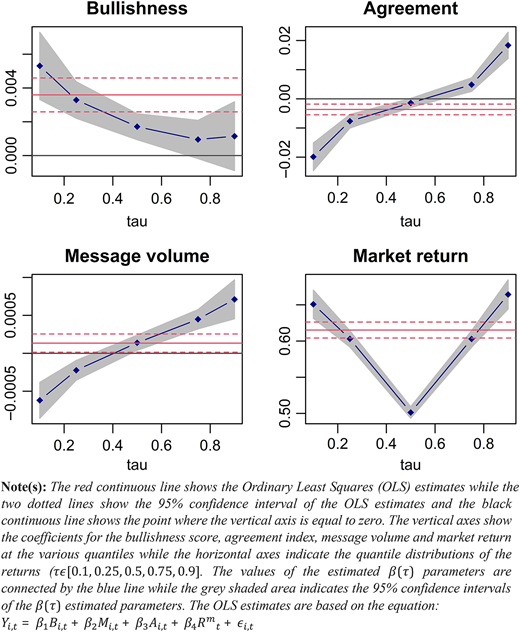
Table 3 shows that bullishness is positively associated with stock returns at all quantiles of stock returns. However, the magnitude of the relationship between bullishness and stock returns persistently falls as we move from the lowest quantile of returns () to the highest quantile of returns (). The coefficients of the relationship fall gradually from in the lowest return quantile to in the highest return quantile. Moreover, the relationship between bullishness and returns becomes less statistically pronounced as we move from the lowest quantile of returns to the highest. The relationship between bullishness and stock returns at the low and middle return quantiles is statistically significant at the 99% confidence level and the significance falls to 90% confidence level at while the relationship at the highest quantile is not statistically significant at any of the conventional confidence levels.
Figure 2 also shows that bullishness falls by increasingly higher margins as we move from lower quantiles of the return distribution but flatten out at higher return quantiles. Textual sentiment extracted from tweets (bullishness) can explain stock market returns under bad and normal market conditions but not under good conditions . This is in line with Allen et al. (2019) who report significantly stronger relationships between textual sentiment extracted from online news articles and stock returns at lower quantiles of the latter. This can be accounted for by more investor decisions being based on stock microblogs around a time when the stock prices are declining than when stock prices are on the rise.
Figure 2 shows that the use of traditional optimisation techniques like the Ordinary Least Squares (OLS) to examine the relationship between stock returns and textual sentiment generally does not reflect the association at extreme market conditions. The OLS estimator only coincides with quantile estimators at and for the remainder of the return quantiles, the coefficients of the bullishness index are outside the 95% confidence interval bands of the OLS estimates. Generally, the results show a monotonic relationship between the magnitude of bullishness and stock returns up to with the relationship becoming flat at the two highest return quantiles .
The results on the relationship between investor agreement and stock returns show three patterns emanating from the quantile distribution of tweet features. Firstly, the estimates increase in absolute terms as we move outwards from the middle quantile to the extreme return quantiles and . Secondly, the coefficients are more significant at lower return quantiles and higher return quantiles while the relationship is less significant at the middle of the return distribution . Thirdly, the relationship between investor agreement and returns is negative (positive) at low (high) return quantiles.
The coefficients (in absolute terms) of the dispersion of investor opinions as measured from tweet messages increases as we move outwards from middle return quantiles to extreme return quantiles. As the quantile levels move up, the estimates of the agreement index vary widely in sign, magnitude and significance. The results are in line with the three hypotheses suggested by Diether et al. (2002) on the association between investor disagreement and stock returns. The authors ascribe the association between agreement and return to three statuses of the overpricing correction process and hypothesise (i) an inverse relationship between agreement and returns when the overpricing is corrected (ii) a positive association between the variables when the overpricing is continuing and (iii) a trivial relationship when the overpricing process is completed. Figure 2 demonstrates three statuses of mispricing correction as the relationship between the agreement index and returns is negative at lower quantiles, positive at upper quantiles and trivial at the middle quantile.
The results show that the conversations on the microblogs largely show disagreements about the prospects of the mentioned tickers at lower quantiles while at higher return quantiles, investors generally agree on the prospects of the companies mentioned on the microblogs. The high dispersion of investor opinions on the microblogs at low return quantiles complements the relationship between bullishness and stock returns at different return quantiles discussed above. Again, the OLS estimate does not capture the relationship between investor agreement and stock returns at the high and low quantiles of the latter.
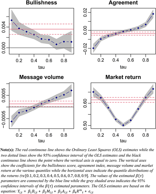
The results on the relationship between the magnitude of message volume and stock returns show that the relationship is significant across all quantiles of returns. However, at low quantiles of returns , the association is negative while at the middle and higher return quantiles, the association becomes positive. As Figure 2 shows, increases in absolute terms as we move from the median quantile to the extreme quantiles and remains statistically significant across all the return quantiles. Like the agreement index, as the quantile levels move up, the estimate of message volume varies widely in sign, magnitude and significance. The 95% confidence intervals of the QR estimates at the very high () and low () quantiles have no overlap with the 95% confidence interval of the OLS estimate. This finding indicates that the OLS estimate does not capture the relation between message volume and stock returns at the high and low quantiles of the latter. For robustness, Figure A1 in the Appendix show similar patterns as indicated above but uses 9 quantiles of returns rather than the 5 used above.
4.4 The information content of past values of tweet features
The contemporaneous relationships between the tweet features and market features discussed in Section 4.2 are crucial in comprehending whether an association between the two exist, but they do not fully portray the quality of the information of past values of firm-level tweets in predicting future returns. Bollen et al. (2011) demonstrate that if microblogs contain new information that is not yet captured by the market prices, tweet features should anticipate the changes in the market features. Granger non-causality tests are appropriate for this cause as they reflect whether past values of a variable have information that can be used to forecast another variable. The results from the panel Granger causality tests on the variables are shown in Table 4.
Pairwise Dumitrescu Hurlin panel causality tests
| Pairwise Dumitrescu Hurlin causality tests | |||||||
|---|---|---|---|---|---|---|---|
| Null hypothesis | W-Stat | Zbar-Stat | p-value | Lags | Causality | ||
| Bullishness | Returns | 1.3739 | 0.5960 | 0.0653 | 1 | NO | |
| Bullishness | Returns | 2.8990 | 0.5960 | 0.1481 | 2 | NO | |
| Agreement | Returns | 1.5673 | 0.7429 | 0.4575 | 1 | NO | |
| Agreement | Returns | 2.4881 | 0.1386 | 0.8897 | 2 | NO | |
| Messages | Returns | 1.3739 | 0.4044 | 0.6859 | 1 | NO | |
| Messages | Returns | 2.8990 | 0.5960 | 0.5512 | 2 | NO | |
| Returns | Bullishness | 3.0226 | 3.2896 | 0.0000 | 1 | YES | |
| Returns | Bullishness | 3.8756 | 1.6832 | 0.0000 | 2 | YES | |
| Returns | Agreement | 3.2555 | 3.6971 | 0.0002 | 1 | YES | |
| Returns | Agreement | 4.8243 | 2.7392 | 0.0062 | 2 | YES | |
| Returns | Messages | 3.0226 | 3.2896 | 0.0010 | 1 | YES | |
| Returns | Messages | 3.8756 | 1.6832 | 0.0023 | 2 | YES | |
Note(s): Null hypotheses: Tweet features (Stock returns) do not homogenously cause Returns (Tweet features)
In line with previous studies which set the rejection criterion at 5%, using one-day lag, the results in Table 4 lead us to fail to reject the null hypothesis that the tweet features do not Granger cause returns. This means that the lagged values of tweet features by one day do not contain important information that could be used to predict stock returns. On the other hand, we reject the null hypothesis that stock returns do not homogenously Granger cause tweet features at the 1% level of significance. This means that the lagged values of stock returns by one day contain useful information that can be used to predict tweet features in the next period. The results using two lags are also qualitatively similar, the tweet features at time do not contain statistically significant and useful information that can be used to predict the stock returns at time . Conversely, it is rather the stock returns at time that contain information that can be used to predict tweet features at time . These results are qualitatively similar to Kim and Kim (2014), who, using panel data and the Granger non-causality method, found no evidence that investor sentiment from internet message boards could predict stock returns either at the individual or aggregate level. Rather, the authors report that investor sentiment extracted from internet message boards through textual analysis is positively affected by previous stock performance. The results from the pairwise Granger causality using weekly data are shown in Table 5.
Pairwise Granger causality tests using weekly data
| Pairwise granger causality tests (weekly data) | |||||||
|---|---|---|---|---|---|---|---|
| Null Hypothesis | Observations | F-statistic | p-value | Lags | Causality | ||
| Bullishness | Returns | 34,045 | 0.99394 | 0.3188 | 1 | YES | |
| Bullishness | Returns | 32,874 | 1.93459 | 0.1445 | 2 | YES | |
| Agreement | Returns | 34,045 | 0.97085 | 0.3245 | 1 | YES | |
| Agreement | Returns | 32,874 | 2.98096 | 0.0508 | 2 | YES | |
| Messages | Returns | 34,045 | 0.01522 | 0.9018 | 1 | YES | |
| Messages | Returns | 32,874 | 0.42453 | 0.6541 | 2 | YES | |
| Returns | Bullishness | 34,045 | 1.04690 | 0.3062 | 1 | YES | |
| Returns | Bullishness | 32,874 | 2.63324 | 0.0719 | 2 | YES | |
| Returns | Agreement | 34,045 | 0.00235 | 0.9614 | 1 | YES | |
| Returns | Agreement | 32,874 | 0.52005 | 0.5945 | 2 | YES | |
| Returns | Messages | 34,045 | 0.52626 | 0.4682 | 1 | YES | |
| Returns | Messages | 32,874 | 0.82600 | 0.4378 | 2 | YES | |
Note(s): Null hypotheses: Tweet features (Stock returns) do not homogenously cause Stock returns (Tweet features)
Using weekly data, the null hypotheses that tweet features do not Granger cause stock returns can be rejected using one week and two-week lags. The results show that weekly tweet features contain useful information that could be used to predict weekly future stock returns. The results in Table 5 also attest to the presence of bidirectional causality between tweet features and stock returns as it can be seen that weekly stock returns also contain important information that could be used to predict future weekly tweet features. The results on the causal relationship between tweet features and stock returns are also similar using monthly data as shown in Table 6.
Pairwise Granger causality tests using monthly data
| Pairwise granger causality tests (monthly data) | |||||||
|---|---|---|---|---|---|---|---|
| Null Hypothesis | Observations | F-statistic | p-value | Lags | Causality | ||
| Bullishness | Returns | 3,238 | 0.25854 | 0.6112 | 1 | YES | |
| Bullishness | Returns | 2,915 | 0.21604 | 0.8057 | 2 | YES | |
| Agreement | Returns | 3,238 | 0.21646 | 0.6418 | 1 | YES | |
| Agreement | Returns | 2,915 | 0.04940 | 0.9518 | 2 | YES | |
| Messages | Returns | 3,238 | 1.12450 | 0.2890 | 1 | YES | |
| Messages | Returns | 2,915 | 3.07479 | 0.0563 | 2 | YES | |
| Returns | Bullishness | 3,238 | 2.5E-06 | 0.9987 | 1 | YES | |
| Returns | Bullishness | 2,915 | 0.02114 | 0.9791 | 2 | YES | |
| Returns | Agreement | 3,238 | 0.00014 | 0.9907 | 1 | YES | |
| Returns | Agreement | 2,915 | 0.60647 | 0.5453 | 2 | YES | |
| Returns | Messages | 3,238 | 0.81981 | 0.3653 | 1 | YES | |
| Returns | Messages | 2,915 | 0.27405 | 0.7603 | 2 | YES | |
Note(s): Null hypotheses: Tweet features (Stock returns) do not homogenously cause Stock returns (Tweet fetures)
Past monthly measures of tweet features have information content that could be used to predict future stock returns using one-month and two-month lags. It can be seen that tweet features have no predictive power on stock returns when using high-frequency daily granularity analysis. At lower weekly and monthly granularity analyses, tweet features are found to be useful in predicting future stock returns. These results provide evidence that might point to cyclical market efficiency on the JSE where the stock market goes through intermittent periods of efficiency and inefficiency. The results also corroborate Seetharam et al. (2017) who document evidence of the dynamic nature of market efficiency on the JSE. The results from the Fama-Macbeth style regressions presented in Tables A3 and A4 in the Appendix corroborate the results from this section.
Lead-lag Fama Macbeth style regressions of returns on tweet features
| Dependent variable | |||
|---|---|---|---|
| Stock returns | |||
| (1) | (2) | (3) | |
| −0.005 (0.007) | |||
| 0.005 (0.007) | |||
| −0.002 (0.003) | |||
| 0.000 (0.000) | |||
| −0.000 (0.000) | |||
| 0.000 (0.000) | |||
| 0.0002*** (0.002) | 0.0002*** (0.002) | 0.0002*** (0.002) | |
| −0.005*** (0.002) | −0.005*** (0.002) | −0.006*** (0.002) | |
| 175,429 | 175,429 | 175,429 | |
| 0.117 | 0.125 | 0.130 | |
Note(s): *p < 0.1; **p < 0.05; ***p < 0.01
The coefficients of the lagged tweets features are all statistically insignificant at the conventional significance levels. Consistent with Sprenger et al. (2014), these results provide evidence that, though tweet features are contemporaneously associated with market features, past values do not contain statistically significant information which can be used to predict future stock returns
Lead-lag Fama Macbeth style regressions of returns on tweet features
| Dependent variable | |||
|---|---|---|---|
| Tweet Features | |||
| Bullishness | Messages | Agreement | |
| 0.115*** (0.017) | −0.327*** (0.148) | −0.031*** (0.010) | |
| 0.071*** (0.016) | −0.273* (0.142) | −0.031*** (0.010) | |
| Size | 0002*** (0.0002) | 0.278*** (0.002) | 0.010*** (0.0001) |
| Constant | −0.048*** (0.006) | −6.233*** (0.056) | −0.214*** (0.003) |
| Observations | 175,253 | 175,253 | 175,253 |
| 0.021 | 0.222 | 0.086 | |
Note(s): *p < 0.1, **p < 0.05, ***p < 0.01
The 1-day and 2-day lagged coefficients of returns are all statistically significant at the 5% level except the 2-day lag coefficient of returns in the model using message volume as the dependent variable. This means that past values of stock returns have useful information that can be used to predict the future values of the tweet features
5. Conclusion
The study purposed to answer three research questions namely; whether there is a contemporaneous link between tweet features and stock market features; whether the magnitude of tweet features is monotonically related to the magnitude of market features; and whether past values of tweet features have information content that could be used to forecast the future values of stock returns. Using the fixed-effects model specification, the study finds that except for the relationship between message volume and stock returns, and between bullishness and stock returns, tweet features are contemporaneously associated with stock market features.
While the results above largely show contemporaneous associations between tweet features and market features at the mean, they do not give a full picture of the rest of the return distribution. On the link between the magnitude of tweet features and stock market features, the findings from the pooled quantile regression show no monotonic link between the magnitude of tweet features and market features. Message volume and investor agreement have stronger relationships with stock returns in absolute terms at extreme return quantiles. The results show no evidence of a monotonic link between the magnitude of tweet features and market features as there are asymmetric spillover effects of tweet features on the stock market returns.
One of the most crucial questions that researchers have grappled with in recent times is whether online messages contain useful content that can be used to predict asset prices. Using panel Granger non-causality tests and lead-lag Fama-Macbeth style regressions, the results from this study show no evidence of past values of tweet features containing important information that could forecast stock market returns in the next period using daily data. The evidence rather shows that stock returns contain useful information that could be used to predict stock market returns in the next period. However, utilising weekly and monthly data, there is strong evidence that historical values of tweet features can be used to predict future returns.
The study examined the link between textual sentiment mined from stock microblogs (Twitter and StockTwits) and market features. However, these market features are only available as aggregate market indicators. Further studies could replace trading volume with the number of trades of different size categories to distinguish between institutional and retail investors since existing literature shows that textual sentiment is mainly associated with individual investors compared to smart investors. Additionally, future research could examine whether the contemporaneous and intertemporal relationships between tweet features and market features are the same in the presence of popular market anomalies.
In conclusion, the study has established no causal effects between the tweet features and the market features using daily granularity. This confirms and implies that the JSE is being dominated by institutional investors rather than noise traders who normally trade on sentiment. Secondly, the lack of causal effects between tweet features and market features at the daily granularity and the existence of the relationship using weekly and monthly data confirms the dynamic nature of efficiency at the JSE. This implies that policymakers have to implement appropriate regulations to deter the development of bubbles or crashes during the “greed” and “fear” cycles. For asset allocation purposes, the findings from this study imply that for a better way of achieving consistent levels of expected returns, active allocation strategies should be dynamic and respond to, and adapt to changing market conditions.
Notes
For the daily bullishness index, we use the scores provided by Bloomberg Inc. which are referred to as Average sentiment scores in the Bloomberg terminal. For all the other tweet features, we use the raw data provided by Bloomberg Inc. for the computations.
References
Appendix 1
Pooled quantile regression estimates with alternative quantiles
| Dependent variable | Independent variables | |||||
|---|---|---|---|---|---|---|
| Stock return | ||||||
| Bullishness | Agreement | Messages | Market return | Constant | Pseudo R2 | |
| 0.1 | 0.005*** (0.001) | −0.019*** (0.00241) | −0.0006*** (0.00012) | 0.651*** (0.0099) | −0.022*** (0.00010) | 0.0426 |
| 0.2 | 0.0037*** (0.001) | −0.0096*** (0.00122) | −0.0002*** (0.00008) | 0.624*** (0.0067) | −0.013*** (0.00007) | 0.0454 |
| 0.3 | 0.0031*** (0.00050) | −0.006*** (0.00100) | −0.0002*** (0.00006) | 0.579*** (0.0054) | −0.007*** (0.00006) | 0.0440 |
| 0.4 | 0.00255*** (0.00043) | −0.0037*** (0.00090) | −0.00002*** (0.00005) | 0.52740*** (0.00443) | −0.0036*** (0.00005) | 0.0440 |
| 0.5 | 0.00171*** (0.00039) | −0.0014*** (0.00079) | 0.00014*** (0.00005) | 0.50134*** (0.00407) | −0.00035*** (0.00004) | 0.0314 |
| 0.6 | 0.00156*** (0.00042) | 0.0004 (0.00084) | 0.00027*** (0.00005) | 0.52345*** (0.00407) | 0.00294*** (0.00005) | 0.0382 |
| 0.7 | 0.00066 (0.00051) | 0.00259** (0.00105) | 0.00040*** (0.00006) | 0.57431*** (0.00495) | 0.00696*** (0.00006) | 0.0423 |
| 0.8 | 0.00118* (0.00065) | 0.0065*** (0.00135) | 0.00052*** (0.00008) | 0.62584*** (0.00667) | 0.01249*** (0.00007) | 0.0433 |
| 0.9 | 0.00115 (0.00104) | 0.0183*** (0.00228) | 0.00071*** (0.00013) | 0.66432*** (0.01026) | 0.02160*** (0.00011) | 0.0380 |
Notes(s): In this Table, for each return quantile, the regression coefficients for each variable are reported and standard errors are shown (in brackets), *p < 0.1; **p < 0.05; ***p < 0.01
Appendix 2
The process of calculating the average sentiment (bullishness) scores used by Bloomberg Inc. starts with manually analysing large datasets of tweets using human experts. Labels are then assigned to each tweet and categorised into positive, negative and neutral labels using the following question:
if an investor having a long position in the security mentioned were to read this tweet, would he/she be bullish, bearish or neutral on his/her holdings
The manually classified feeds are then fed into machine learning models that are taught to imitate language experts in analysing text messages. The completed machine learning models are subsequently used to scrutinise new tweets tagged with tickers and assign each tweet a story-level sentiment score ranging from −1 to +1 in real-time. Bloomberg does not, however, disclose the details of the models used to determine the sentiment scores because of their proprietary nature. The average firm-level daily sentiment (bullishness) is then extracted from the weighted average story-level sentiment scores in the last 24 h collected from Twitter and StockTwits and updated every day 10 min before the JSE opens and is calculated as:
where:
is the bullishness score for firm at time ;
is the sentiment polarity score for tweet that references firm ;
is the confidence of tweet that references firm ;
is the set of all non-neutral tweet feeds that reference firm in the 24 hour-period, T;
is firm total number of positive or negative tweets during period T.
