An Introduction to Regression & Canonical Commonality Analyses: Partitioning Predicted Variance into Constituent Parts

Middle-grades researchers frequently utilize multiple regression analyses to predict or explain relationships between variables such as student motivation or perceived educational value and academic achievement (see Capraro & Capraro, elsewhere in this volume). In multiple regression analyses, in addition to a noteworthy effect size (consider Thompson or Zhang elsewhere in this volume), researchers are interested in defining the relative contribution of each predictor to the overall effect. For example, in the case that student motivation and perceived educational value together are good predictors of academic achievement, researchers may want to investigate the unique contributions of each of these variables or their shared contribution to the prediction to improve theory. As emphasized by Seibold and McPhee (1979),

Advancement of theory and useful explanation of research findings depend not only on establishing that a relationship exists among predictors and the criterion, but also upon determining the extent to which those independent variables, singly and in all possible combinations, share variance with the dependent variable. (p. 355)

In this paper, commonality analysis is introduced to middle-grades researchers as a way to partition the variance within the outcome (i.e., dependent) variable to determine the proportions of variance that (a) are uniquely accounted for by each predictor (i.e., independent variable) (or predictor set) and (b) are commonly accounted for by all possible combinations of predictors (or predictor sets) (Pedhazur, 1982).

Commonality analysis was originally developed for use in multiple regression analysis, and it partitions the explained variance in the outcome variable to “understand the relative predictive power of the regressor variables, both individually and in combination” (Beaton, 1973, p. 2). The extension of commonality analysis to multivariate analyses has also been illustrated by various researchers (Beaton; Thompson & Miller, 1985).

When the predictors are perfectly uncorrelated, there is no shared contribution between any predictors, and each predictor’s unique contribution to the model is equal to the squared correlation (r²) between that predictor and the outcome variable. However, in real research data are often correlated so inference about predictors’ unique and common contributions can be difficult. In the latter case, commonality analysis facilitates result interpretation by quantifying every unique and common contribution to prediction.

To prevent any possible confusion it is important to note commonality analysis is different from the interaction effect analysis in OVA models. According to Thompson (2006, p. 293) “Interaction effects quantify the degree to which predictors or independent variables perform differently in the presence of the other predictors, thereby creating unique additional effects through their joint functioning.” In a balanced ANOVA design, interaction effects are perfectly uncorrelated with the main effects. On the other hand, commonality is the shared contribution between two or more predictors. For example, if predictors A and B share a common contribution, this common explanatory power exists in both A and B, and including either A or B alone in the model will bring this same explanatory power to the model.

Commonality analysis is an alternative to stepwise analyses to evaluate predictors’ relative contributions. Researchers incorrectly think that the entry order of predictors for stepwise regression yield the predictors’ relative contributions (Zientek & Thompson, 2006). Another common erroneous belief about stepwise is that it provides the optimal R² for a given set of predictors. However, the incremental selection process employed by stepwise (i.e., choosing the best predictor given the ones already in the model) does not necessarily yield the set of predictors at a certain size with the largest R² (Thompson, 2006). In reality, another set of predictors may provide a better R², and further, that optimal predictor set may not contain any of the predictors selected by the stepwise method. Commonality analysis provides better insight into each predictor’s relative predictive power.

The present paper’s purpose is to explain and demonstrate commonality analysis to provide middle-grades researchers with a reporting option, to foster theory building, and as a means of developing more parsimonious models. First, commonality analysis in a multiple regression context is explained followed by a generalization of commonality analysis to canonical correlation analysis (CCA). Heuristic applications of commonality analysis in both univariate and multivariate cases using SPSS are discussed.

Commonality analysis improves result interpretation by determining predictors’ unique and common contributions to the regression model. A predictor’s unique contribution is the proportion of variance incremented when that predictor is the last variable entered in the regression (Pedhazur, 1982). On the other hand, the common contribution (i.e., commonality) of a group of predictors is the proportion of variance that can be explained using any one of the predictors in that specific group.

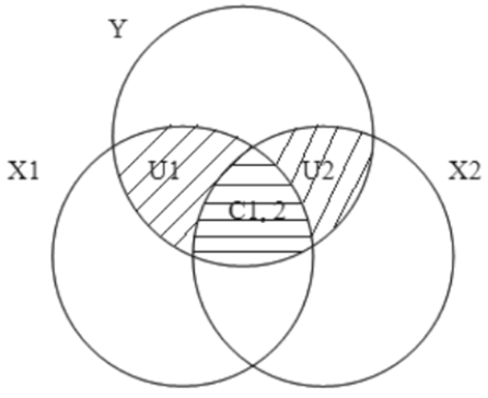
To make the discussion concrete, presume a regression case involving two correlated predictors. Figure 1 shows a Venn diagram for this hypothetical case, where Y is the outcome and X1 and X2 are two predictor variables. The hatched area represents the explained variance in Y by X1 and X2. The purpose of the commonality analysis is to determine the explained variance unique to X1 (i.e., U1), unique to X2 (i.e., U2), and common to both predictors (i.e., C(1,2)).

The unique contribution of X1 can be obtained as

U1 = R² (12) - R² (2) (1)

where U1 is the unique contribution of X1, R² (12) is the squared multiple correlation of Y with X1 and X2, and R² (2) is the squared multiple correlation of Y with X2. In a similar fashion, the unique contribution of X2 is

U2 = R² (12) - R² (1) (2)

where U2 is the unique contribution of X2, and R² (1) is the squared multiple correlation of Y with X1. As a general rule for regressions with any number of predictors, the unique contribution of each predictor is equal to the difference in R² between the model with all of the predictors and the model with only the predictor of interest missing. In the present example, the common contribution of X1 and X2 can be found by subtracting the unique components from R² (12): C(1,2) = R² (12) - U1- U2.

To compute commonality coefficients, all possible combinations of R² are required. For instance, in the above example R² (1), R² (2), and R² (12) were all used to obtain the unique and common contributions. Appendix A presents the necessary formulas for all commonality coefficients when two, three and four predictors are involved. An exponential function represents the number of components for which R² can be decomposed. If there are p predictors in a regression model, the number of commonality coefficients to be calculated is 2^P-1, p unique variance components, and (2^P-1)-p commonalities.

In this section, to make the computations of commonality analysis concrete and to illustrate the use of SPSS for commonality analysis, a scenario relevant to middle-grades researchers is presented. For this scenario, real data collected by Holzinger and Swineford (1939) from seventh- and eighth-grade children on 26 psychological measures are used. For the current scenario 4 of these 26 test results are used: paragraph comprehension test scores (T6), word classification test scores (T8), mathematics word problem reasoning test scores (T22), and word meaning test scores(Y). Middle-grades researchers may want to predict the seventh- and eighth-grade students’ word meaning test scores (Y) using their scores on paragraph comprehension (T6), word classification (T8), and mathematics word problem reasoning (T22) tests. Thus, in a regression model the outcome variable is Y, and predictors are T6, T8, and T22.

In such a regression model, a middle-grades researchers’ first interest would be to determine the statistical and practical significance of the effect size (R²). In the current scenario, R² was found to be 0.571. If (and only if) the researcher decides the obtained effect (R²) is meaningful, he or she might be interested in predictors’ relative importance (Thompson, 2006). For example, the researcher might want to know the unique contribution of mathematics word problem reasoning to the prediction or the shared contribution of mathematics word problem reasoning and word classification. These and similar questions about predictors’ unique and shared contributions can be answered using commonality analysis.

The commonality analysis in the current scenario with three predictor variables would result in 2³ - 1 = 7 variance components that explain (a) each predictor’s unique contribution (i.e., U6, U8, and U22), (b) contributions common to two predictors (i.e., C(6,8); C(6,22); and C(8,22)), and (c) contribution common to all three predictors (i.e., C(6,8,22)). The commonality analysis starts with obtaining all possible combinations of R². Accordingly, several multiple regression analyses are conducted to predict the outcome variable (i.e., word meaning) using the predictors individually (i.e., R² (6), R² (8), R² (22)) and in all possible combinations with each other (i.e., R²(6,8), R²(6,22), R² (8,22), R² (6,8,22)). The necessary syntax to get the required R² values for the current scenario with three predictors is presented in Appendix B.

Once the needed R² values are obtained, they are placed into relevant commonality-coefficient formulas to obtain predictors’ unique and common contributions. For example, the predictive contribution common to paragraph comprehension and word classification (i.e., C(6,8)) can be calculated as

C(6,8) = - R² (22) + R² (6,22) + R²(8,22) - R² (6,8,22)

= -0.256 + 0.542 + 0.426 - 0.571

= 0.141

= 14.1%.

Table 1 presents all seven components of explained variance in the outcome variable, word meaning. This tabular form facilitates interpretation and allows for an arithmetic check of the computations. The sum of the columns for each predictor is equal to the correlation between that predictor and the outcome variable. For example, the correlation (i.e., r²) between paragraph comprehension (T6) and word meaning (Y) is 49.6%, which is also equal to the R² of the regression model where T6 is the only predictor entered into the model. Also, the last column of the table, the sum of the seven partitions, adds up to the total variance explained (57.1%).

In the current scenario, test scores on paragraph comprehension had the highest unique contribution (i.e., U6 = 14.5%) to the prediction of word meaning test scores. The other predictors had little unique contributions (i.e., U8 = 2.9%, U22 = 3.0%) but large commonalities with other predictors (i.e., C(6,8) = 14.1%, C(6,8,22) = 15.2%). In fact more than half of the explanatory power of mathematics word problem reasoning was common to all three predictors (C(6,8,22) = 15.2%).

Canonical correlation analysis (CCA) is employed to investigate the relationship between two sets of variables, each of which contain at least two variables (Thompson, 1984). CCA is the most general case in the GLM model subsuming almost all univariate and multivariate parametric analyses (e.g., t-test, ANOVA, multiple regression, MANOVA) as special cases (Knapp, 1978), and CCA can replace numerous univariate tests and provides a more accurate real-world model where dependent variables are almost always related. Further, Thompson (1988) illustrated how CCA can be used to implement the univariate and multivariate parametric tests. In the same paper, Thompson suggested that because multiple regression is a special case of CCA, commonality analysis used in the interpretation of regression results can also facilitate interpretation of CCA results.

In this section, the multivariate extension of commonality analysis to CCA is illustrated using the Holzinger and Swineford data set. One more variable from the data set, namely Woody-McCall mixed mathematics fundamentals test (T24), is added to the variables used in the above regression commonality analysis. For the CCA application, researchers are interested in the relationship between two sets of variables. The first set, named as criterion (one can think of these as dependent) variables, consists of Woody-McCall mixed mathematics fundamentals test (T24) and word meaning test scores (T9). The second set, named as predictor variables, consists of paragraph comprehension test scores (T6), word classification test scores (T8), and mathematics word problem reasoning test scores (T22).

Canonical correlation analysis is utilized to investigate the relationship between two sets of variables. Before proceeding with commonality analysis, canonical correlation coefficients (R_cs) are obtained. The number of R_cs produced in a CCA is equal to the number of variables in the smaller set. Each R_c is computed based on a canonical correlation function. In the current scenario, because the smaller set has two variables (i.e., criterion variables), CCA resulted in two R_cs based on two different canonical correlation functions. The canonical correlation coefficient for the first function was 0.780, and the squared canonical correlation coefficient (R_c²) was 0.608 (because 0.608 = 0.780²). Because procedures to partition the squared canonical coefficient are the same for every function, the commonality analysis illustration is done only on one function.

The commonality analysis for the current CCA allows partitioning the explained variance in the criterion variables set (R_c² = 0.608) to determine (a) unique contributions of each predictor (i.e., U6, U8, and U22), (b) contributions common to two predictors (i.e., C(6,8); C(6,22); and C(8,22)), and (c) contribution common to all three predictors (i.e., C(6,8,22)). The CCA commonality analysis starts with creating a composite score, also called canonical variates, for the criterion variables. In effect, canonical variates can be obtained for both sets (i.e., criterion and predictor). However, for this commonality analysis, only the criterion variate scores are needed, so the variate scores for the predictor variables will not be computed. The canonical variates (CRIT 1; name used in the syntax) are obtained by applying standardized canonical function coefficients to the standardized (i.e., z-scores) criterion variables. Table 2 presents the correlation matrix for all the variables and the canonical function coefficients for the first function. Below is an illustration of variate score computation for the first participant:

(0.275 * ZT24) + (0.848 * ZT9) = (0.275 * -0.05613) + (0.848 * -0.82134)

= -0.71

The variate scores are computed for each person in a similar fashion.

After the canonical variates are obtained for the criterion variables (i.e., CRIT1), several multiple regression analyses are conducted to predict CRIT1 using predictor variables individually (T6, T8, and T22) and in all possible combinations with each other ((T6,T8), (T6,T22), (T8,T22), and (T6,T8,T22)). The necessary syntax to get the required R² values and also to run all the previous processes in the previous steps of canonical commonality analysis is presented in Appendix C.

Once the needed R² values are obtained, these R² values are placed into relevant commonality coefficients formulas to obtain all the unique and common contributions of the predictor variables. Table 3 presents all seven canonical uniqueness and commonality estimates. It is important to note that the multiple correlation coefficient when all predictors are entered simultaneously (i.e., R² = 0.608) equals the squared canonical correlation coefficient, because the two analyses are equivalent. Another observation is because we partitioned the squared canonical correlation, the sum of the seven partitions add up to .608.

For these data, paragraph comprehension test scores (T6) had the highest unique contribution (i.e., U6 = 13.9%) to the canonical model. The other predictors had little unique contributions (i.e., U8 = 3.4%, U22 = 4.1%) but large commonalities with other variables (i.e., C(6, 8) = 14.5%, C(6, 8, 22) = 16.7%). In fact, nearly half of the predictive power of word classification test scores (T8), and mathematics word problem reasoning test scores (T22) was common to all three predictors. Therefore, T6 alone should be retained for future studies.

Middle grades researchers can develop more powerful theoretical models through commonalty analysis that disclose unique and common contributions of predictors to the model. This allows future researchers to choose among variables to select the most parsimonious model. By selecting the most parsimonious models researchers can control both financial costs to collect data as well as participant costs in terms of time.

However, commonality analysis has some limitations. The number of commonalities increases rapidly as the number of independent variables increases thereby complicating the interpretation of especially higher order commonalities. Researchers can overcome this constraint by limiting the number of variables to the commonly recommended number of four or by grouping the variables based on theory or through methods such as cluster analysis or factor analysis (Seibold & McPhee, 1979).

Another possible problem in commonality analysis is negative partitions. The unique partitions cannot be negative but the partitions that are common to two or more predictors can have negative signs. These negative commonalities can occur due to sampling error or suppressor effects. Negative commonalities can also be obtained when some of the correlations between the predictors are positive and some are negative (Pedhazur, 1982). If the negative values are near-zero, they are generally treated as zeros. If they are large, then the results are considered unacceptable, and the aforementioned possible reasons of negative partitions should be investigated (Thompson, 2006).

Finally, a cited drawback of commonality analysis is there are no statistical significance tests for commonality analysis. However, this disadvantage is not substantial, because commonality analysis is conducted only after a statistically significant effect size has been found (consider Thompson elsewhere in this volume).

Formulas for Unique and Common Components of Explained Variance

Two Independent Variables

U1 = - R² (2) + R² (12)

U2 = - R² (1) + R² (12)

C12 = R² (1) + R² (2) - R² (12)

Three Independent Variables

U1 = - R²(23) + R²(123)

U2 = - R²(13) + R²(123)

U3 = - R² (12) + R² (123)

C12 = - R²(3) + R²(13) + R²(23) - R²(123)

C13 = - R²(2) + R²(12) + R²(23) - R²(123)

C23 = - R²(1) + R²(12) + R²(13) - R²(123)

C123 = R²(1) + R²(2) + R² (3) - R²(12) - R²(13) - R²(23) + R²(123)

Four Independent Variables

U1 = - R²(234) + R²(1234)

U2 = - R²(134) + R²(1234)

U3 = - R² (124) + R² (1234)

U3 = - R²(123) + R²(1234)

C12 = - R²(34) + R²(134) + R²(234) - R²(1234)

C13 = - R² (24) + R²(124) + R²(234) - R²(1234)

C14 = - R²(23) + R²(123) + R²(234) - R²(1234)

C23 = - R²(14) + R² (124) + R²(134) - R²(1234)

C24 = - R²(13) + R²(123) + R²(134) - R²(1234)

C34 = - R²(12) + R²(123) + R²(124) - R²(1234)

C123 = - R²(4) + R²(14) + R² (24) + R²(34) - R²(124) - R²(134) - R² (234) + R² (1234)

C124 = - R²(3) + R²(13) + R²(23) + R²(34) - R²(123) - R²(134) - R²

(234) + R² (1234)

C134 = - R²(2) + R²(12) + R² (22) + R² (24) - R²(123) - R²(124) - R² (234) + R² (1234)

C234 = - R²(1) + R²(12) + R²(13) + R² (14) - R²(123) - R² (124) - R²

(134) + R² (1234)

C234 = R²(1) + R²(2) + R² (3) + R²(4) - R² (12) - R²(13) - R² (14) - R² (23) - R² (24) -R² (34) + R²(123) + R²(124) + R²(134) + R² (234) - R² (1234)

REGRESSION VARIABLES = T6 T8 T22 Y

/STATISTICS = R, COEFF ANOVA /DEPENDENT = Y

/METHOD = ENTER T6 T8 T22.

REGRESSION VARIABLES = T6 T8 T22 Y /DEPENDENT = Y/ENTER T6 T8 T22.

REGRESSION VARIABLES = T6 T8 T22 Y /DEPENDENT = Y/ENTER T6 .

REGRESSION VARIABLES = T6 T8 T22 Y /DEPENDENT = Y/ENTER T8 .

REGRESSION VARIABLES = T6 T8 T22 Y /DEPENDENT = Y/ENTER T22 .

REGRESSION VARIABLES = T6 T8 T22 Y /DEPENDENT = Y/ENTER T6 T8 .

REGRESSION VARIABLES = T6 T8 T22 Y /DEPENDENT = Y/ENTER T6 T22 .

REGRESSION VARIABLES = T6 T8 T22 Y /DEPENDENT = Y/ENTER T8 T22 .

subtitle ‘Run Canonical Analysis using SPSS MANOVA Command’ . MANOVA

T24 T9 WITH T6 T8 T22

/PRINT = SIGNIF (MULTIV EIGEN DIMENR)

/DISCRIM = (STAN ESTIM COR) .

DESCRIPTIVES

VARIABLES = T24 T9 /SAVE

/STATISTICS = MEAN STDDEV .

COMPUTE CRIT1 = (.275*Zt24) + (.848*Zt9) .

Subtitle ‘1A REGRESSION TO PRED CANONICAL SYN WITH 3

PREDS’ .

REGRESSION VARIABLES = CRIT1 T6 T8 T22/

DEPENDENT = CRIT1/ENTER T6 T8 T22 .

Subtitle ‘2A REGRESSION TO PRED CANONICAL SYN WITH 2

PREDS’ .

REGRESSION VARIABLES = CRIT1 T6 T8 T22/

DEPENDENT = CRIT1/ENTER T6 T8 .

Subtitle ‘3A REGRESSION TO PRED CANONICAL SYN WITH 2

PREDS’ .

REGRESSION VARIABLES = CRIT1 T6 T8 T22/

DEPENDENT = CRIT1/ENTER T6 T22 .

Subtitle ‘4A REGRESSION TO PRED CANONICAL SYN WITH 2

PREDS’ .

REGRESSION VARIABLES = CRIT1 T6 T8 T22/

DEPENDENT = CRIT1/ENTER T8 T22 .

Subtitle ‘5A REGRESSION TO PRED CANONICAL SYN WITH T6’ .

REGRESSION VARIABLES = CRIT1 T6 T8 T22/

DEPENDENT = CRIT1/ENTER T6 .

Subtitle ‘6A REGRESSION TO PRED CANONICAL SYN WITH T7’ .

REGRESSION VARIABLES = CRIT1 T6 T8 T22/

DEPENDENT = CRIT1/ENTER T8 .

Subtitle ‘7A REGRESSION TO PRED CANONICAL SYN WITH

T14’ .

REGRESSION VARIABLES = CRIT1 T6 T8 T22/

DEPENDENT = CRIT1/ENTER T22 .