


This study aims to assist researchers in achieving accurate predictions of stabilized soil properties using artificial neural networks (ANNs). It also highlights and documents the limitations of existing studies, while presenting suggestions and potential directions for future advancements.
This study explores the extensive application of ANNs in predicting soil characteristics, with a particular focus on stabilized soils. A structured framework (PRISMA) was used for the systematic selection and refinement of the literature. Over a hundred published articles related to ANNs in the field of soil stabilization were reviewed, and the key insights were identified. The processes involved in the ANN analysis, such as the collection of data required, the network architecture, the performance of the model and the sensitivity analysis, will be briefly discussed. This approach is expected to serve as a valuable reference for researchers pursuing work in this area.
The findings from the study indicate that ANN is a reliable tool for accurately predicting the mechanical properties of soil. One notable shortcoming in the reviewed studies is the lack of specification regarding clay mineralogy. Since the properties of the soil depend on clay mineralogy, the developed ANN models without the specifications of clay mineralogy and soil type cannot be regarded as impartial predictors. The stabilized soil properties like permeability coefficient, consolidation characteristics, resilient modulus and free swelling potential found limited in research and require further exploration. Future research should also address the influence of climatic variations on stabilized soil behavior and explore the integration of other machine learning approaches to enhance predictive capabilities.
This study can serve as a guide for researchers interested in predicting the properties of stabilized soils using ANNs. It also identifies existing research gaps and provides possible suggestions for addressing them.
1. Introduction
The management of problematic soils poses serious difficulties in the field of civil engineering (Mohamad et al., 2015) as they often lack the stability needed to support foundations for structures (Bell, 1993; Kang et al., 2015). For instance, in the earthen dam construction, the suitability of clayey soil for the core material of an earthen dam could become doubtful if it is dispersive soil (Vakili et al., 2015). Hence, safe construction over such problematic soil without ground improvement is infeasible. Various techniques for improving the problematic ground include surface compaction, grouting, preloading with vertical drains, mixing the soil with admixtures, thermal/freezing method, soil reinforcement methods such as using geosynthetics, soil nailing and stone columns. The selection of a suitable ground improvement method is a challenging part for geotechnical engineers. The proper choice of ground improvement technique leads to an economical solution to any problematic soil.
Soil stabilization is an important ground improvement technique that aids in achieving the desired properties of the soil (Aparna et al., 2019). Enhancement of soil properties by soil stabilization can be achieved by chemical stabilization, geosynthetic stabilization or geopolymer stabilization. One approach to soil stabilization, chemical stabilization, improves soft soil properties by increasing its shear strength (Kang et al., 2015). Adding a chemical additive could significantly change clayey soil’s physical, chemical and mechanical properties (Indraratna et al., 1991; Verma et al., 2021). Chemical additives will also help to reduce maintenance costs (Cabezas and Cataldo, 2019) and improve the stability and stiffness of soil (Barman and Dash, 2022). Chemical stabilization strengthens expansive soils by enlarging particle size and boosting soil cementation properties, reducing the plasticity index and swelling-shrinkage potential (Zada et al., 2023). This technique helps the problematic soil to meet its engineering project requirements (Kolias et al., 2005). For chemical stabilization, materials such as Cement, CC (Pandey and Rabbani, 2017); Lime, L (Rajasekaran and Narasimha Rao, 2000); waste by-products such as Fly Ash, FA (Ahmad et al., 2015); Sewage Sludge Ash, SSA (Aparna, 2022); Rice Husk Ash, RHA (Basha et al., 2005); Pond Ash, PA (Kolay et al., 2011); Cement Klin Dust, CKD (Miller and Azad, 2000); Plastic Wastes, PW (Gangwar and Tiwari, 2021); Ground Granulated Blast Furnace Slag, GGBFS (Abdila et al., 2022); and Quarry Dust, QD (Suits et al., 2005) are commonly used. Geosynthetic stabilization can be achieved using products such as Geotextiles, GT (Ogundare et al., 2018); Geomembranes, GM (Elgamal and Adalier, 1996); Geogrids (Esmaeili et al., 2018) and Geocells (Song et al., 2021). The geo-polymerization process involves the activation of alumino-silicate minerals present in the soil or added materials (like fly ash or slag) with an alkaline solution, forming Geopolymers, GP (Ghadir and Ranjbar, 2018). The geopolymers are excellent binders that stabilize the soil. Assessing the performance of stabilized soil is essential, regardless of the type of stabilizer used, to confirm its suitability for construction applications.
Soil properties can indeed vary significantly across different locations (Ngo et al., 2021) and even within the same area. Several factors, such as climate, topography, parent material, weathering time and soil type, can influence the variability. The properties of stabilized soil are also governed by these factors, making it a complex multivariable issue that demands comprehensive analysis (Jeremiah et al., 2021). Therefore, applying an existing empirical formula to predict the properties of stabilized soil may not be reliable. The various factors responsible for soil variability can contribute to the differences in soil texture, structure, composition, moisture content, pH, index properties, engineering properties and the degree of improvement of soil by the addition of any additives. These values are mostly determined by laboratory studies (Ngo et al., 2021). Laboratory testing is a critical phase in determining engineering and index properties for stabilized or unstabilized soil as per standard procedures. These results help to identify the soil type available on the site. The performance of the stabilized soil is analyzed using parameters like unconfined compressive strength (UCS), permeability (k), resilient modulus (Mr), California bearing ratio (CBR), optimum moisture content (OMC) and maximum dry density (MDD) (Chew et al., 2004; Alavi et al., 2009). Although laboratory studies provide geotechnical engineers with dependable results, they are often time-consuming, labor-intensive and costly (Bahmed et al., 2017).
Artificial intelligence (AI) can be described as the “science and engineering of making intelligent machines” (Collins et al., 2021). Deep learning (DL), artificial neural networks (ANNs) and machine learning (ML) are subsets within the broader field of AI. In recent years, the use of ML techniques has shown significant promise for addressing a broad spectrum of challenges in geotechnical engineering (Es-haghi et al., 2023). The application of ML approaches to predict the properties of stabilized soil offers cost and time reductions compared to experimental studies. Therefore, ML can be used to forecast the engineering properties of stabilized soil. The major contribution of this review includes a fundamental idea of ML and its application in geotechnical engineering; a basic idea of ANN and its utilization in geotechnical engineering; a detailed systematic review of the application of ANN in soil stabilization and the step-by-step process which comprises of data collection, data preprocessing, model training, model performance and sensitivity analysis; finally, the summary and conclusion section concludes this review, and the promising topics for future research will be highlighted. This review will support developers and researchers in expanding their understanding of applying ANNs to soil stabilization.
2. Machine learning and its application in geotechnical engineering
AI encompasses a range of scientific definitions, but it generally refers to systems or applications that can execute tasks requiring human-like perception and decision-making (Rai et al., 2019; Longoni et al., 2019). Along with ML and DL, the field of AI also includes computer vision and natural language processing (NLP). AI’s presence is growing across various technological sectors because it enables rapid advancements. The application of AI in civil engineering (Huang et al., 2019) and Geotechnical engineering (Baghbani et al., 2022) has been reviewed by various researchers.
Even though ML is a specific type of AI (Soori et al., 2023), not all AI incorporates machine learning. ML algorithms excel at analyzing data to identify patterns and make predictions, but they cannot address broader issues or be adapted as flexibly as AI. By learning from data and making informed decisions, ML has revolutionized how computers perform tasks, automating processes that were once thought to require human intelligence. ML, known for including powerful techniques, is now being used more frequently by geotechnical engineers. Common ML approaches include ANN (Khatti and Grover, 2021; Krishna et al., 2023; Ouf, 2012; Nagaraju et al., 2023), Functional Network (FN) which is an advanced version of ANN (Das et al., 2011), Multivariate Adaptive Regression Splines (MARS) (Samui et al., 2015), Regression Analysis (RA), Gaussian Process Regression (GPR), Relevance Vector Machine (RVM) (Khatti and Grover, 2021), Adaptive Neuro-Fuzzy Inference System (ANFIS) (Walia et al., 2015; Samui et al., 2015),Fuzzy Inference System (FIS) (Jouffe, 1998), Genetic Algorithms (GA) (Narendra et al., 2006; Kumar et al., 2010; Ouf, 2012), Particle Swarm Optimization (PSO) (Settles, 2005), Support Vector Machine (SVM) (Das et al., 2011; Khatti and Grover, 2021; Zhang et al., 2023), K-Nearest Neighbor (KNN), Random Forest (RF), Decision Tree (DT) (Zhang et al., 2023), Gradient Boosting (GB) (Ngo et al., 2021; Zhang et al., 2023) and DL (Xu et al., 2021). Within these techniques, the most widely used ML approach in geotechnical engineering is the ANN (Baghbani et al., 2022), which shows high accuracy and is economical compared to experimental studies (Suman et al., 2016). A comparative study by Kumar and Harinder (2020) on soil stabilization demonstrated that ANNs outperform SVMs in predicting soil properties.
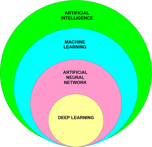
ANNs are computational models in ML designed to simulate how the human brain processes information. Although several general-purpose data-driven techniques exist, ANNs are among the most commonly used methods for pattern recognition (Rezania et al., 2008; Javadi and Rezania, 2009). The structure of an ANN is modeled after the human nervous system (HNS) (Shahin et al., 2001). DL, a specialized field within ML, uses neural networks to replicate the cognitive processes of the human brain. As one of AI’s most advanced tools, DL demonstrates remarkable capability in mapping complex nonlinear relationships across fields, including civil engineering (Lazarevska et al., 2014) and early warnings in geotechnical engineering (Chou and Thedja, 2016). DL falls under the broader ANN with many layers. Thus ANN, used in DL, is a type of ML that helps computers learn from a massive volume of data (Howard, 2019). Serving as the key tool in DL, ANN has been widely applied in various geotechnical areas (Zhang et al., 2023). A diagrammatic representation of AI, ML, ANN and DL is shown in Figure 1.
While other ML techniques such as SVM, Random Forests (RF), Adaptive Neuro-Fuzzy Inference Systems (ANFIS) and long short-term memory networks (LSTM) have been successfully applied in geotechnical engineering, their use in soil stabilization remains comparatively limited. The key features of SVM include the use of kernel functions, the sparsity of the solution, the absence of local minima and capacity control achieved through either the margin or the number of support vectors (Tabarsa et al., 2021). RF is advantageous for handling high-dimensional data sets with relatively low computational cost (Adugna et al., 2022), while ANFIS offers interpretability by combining fuzzy logic with neural networks (Sinha and Tiwari, 2025). LSTM, a DL architecture, shows promise for time-dependent geotechnical processes but requires large data sets and higher computational resources (Mojtahedi et al., 2025). In contrast, ANN has been most widely applied to stabilized soils due to its flexibility, relative ease of implementation and ability to approximate nonlinear relationships even with moderately sized data sets. This review mainly concentrates on ANN, while recognizing that hybrid or ensemble approaches integrating ANN with other models may yield enhanced performance in future studies. A recent study by Sangdeh et al. (2024) obtained from their study that hybrid ANN-PSO model shows the best performance for the prediction of UCS and precipitated calcium carbonate (PCC) values for microbially induced calcite precipitation (MICP) mediated soils. Several researchers have enhanced the performance of ANNs by integrating GAs, which help optimize model parameters, reduce overfitting and enhance the model’s generalization ability (Katoch et al., 2021; Wang et al., 2024).
3. ANN and its application in geotechnical engineering
ANN models include all the necessary physical components of the brain, aiming to replicate its complex functionalities (Kalkan et al., 2009). In HNS, dendrites gather information (analogous to input in ANN), transfer it to the nucleus (similar to hidden layers in ANN) for processing and generate synapses (comparable to outputs in ANN). Similar to human learning, ANNs also learn through training. However, it should be noted that computational neuroscience works on extremely accurate and complex phenomena. Hence, an artificial neuron is just a toy case of a biological neuron. Essentially, ANNs serve as automated optimization systems that learn the relationships between various input variables and model these relationships using trends and patterns in mathematical functions, facilitating accurate predictions or output (Steniewska-Dziubinska et al., 2018). Non-linear mapping facilitates the connection between input and output data (Were et al., 2015). ANN modeling is a potential tool for non-linear problem prediction (Naghibi et al., 2016). Hubick suggested that ANNs are well-suited for modeling intricate problems, particularly when the connections between variables are not explicitly known (Hubick, 1992).
Depending on their learning methods, ANNs are categorized into hybrid, unsupervised and supervised learning categories. Supervised (discriminative) learning involves training a network with known input and target values. The primary difference between regression and classification algorithms lies in their outputs: regression predicts continuous variables like salary, price or age, while classification assigns discrete labels, such as gender, spam/not spam or true/false. Conversely, unsupervised ANNs are trained using an iterative approach of trial and error. Here, unknown output or target parameters are predicted using known input parameters. Grouping of such unlabeled examples is known as clustering. Hybrid (reinforcement) learning blends elements of both unsupervised and supervised learning (Sarkar, 2021).
Various types of ANNs have a wide range of applications, including data classification, prediction, conceptualization and filtering (Salahudeen et al., 2018). Based on their structure, ANNs are classified into Recurrent and Feed-forward networks (FFN). Recurrent Neural Networks (RNN) are bi-directional, in which the output of one layer is stored and fed back into the input, allowing for improved prediction of the layer’s result. Feed forward network (or) a simple neural network (or) a multilayered neural network is basically a collection of neurons where the connections are fed forward without any cycle or loop. Here, the flow of information is unidirectional, moving from the input nodes through the hidden layer and toward the output layer. The major feed-forward ANN architectures include single-layer perceptron (SLP), mainly for linearly separable problems, convolutional neural networks (CNN or ConvNet) and multi-layer perceptron (MLP). Based on their training algorithms, ANNs can be classified into backpropagation networks, BPN (type of FFN), Hopfield networks (type of RNN) and self-organizing map networks (type of unsupervised ANN). (Chao et al., 2018).
Among feed-forward networks, the Multilayer Perceptron (MLP) is the preferred choice for addressing both classification and regression problems (Erzin et al., 2009; Alavi et al., 2010; Vakili et al., 2015). As universal approximators, MLP networks are capable of approximating any continuous function to remarkable precision. Supervised learning tasks frequently use these networks, using iterative methods to adjust connection weights during training. MLP networks are commonly trained using the backpropagation algorithm (BPA) (Rumelhart et al., 1986). Backpropagation (BP) efficiently adjusts weights in feedforward networks with differentiable activation units, enabling learning from a training data set of input-output pairs (Castro, 2007). This training algorithm includes feed-forwarding the values, calculating the error and propagating it back. In this, by reorganizing weights and comparing predicted and target values, the error will be reduced to a minimum.
ANNs are a collection of interconnected nodes or “neurons” that process data in layers, to perform tasks by adjusting the connections (weights) based on the data they process. Figure 2 presents a feed-forward ANN integrated with the BPA. The multilayered perceptron (Figure 2) consists of layers arranged in succession, with each layer forming a parallel system of interconnected units, acting as elementary processors. The input layer is made up of nodes (or neurons) that accept the input features from the data set. Each input node corresponds to a feature in the input data. The layers in the middle, called hidden layers, carry out the necessary computations. These hidden layers can consist of a single layer (shallow network) or multiple layers (deep neural network) (Ikizler et al., 2009). The output layer, which is the final layer, produces the results based on the computations carried out by the hidden layers. The number of nodes in this layer corresponds to the number of output variables (Vakili et al., 2015).
 The diagram shows a neural network framework for forward and backward propagation. Five inputs labeled as Input 1 to Input 5 connect to a hidden layer through various weights denoted as W1 to W18. The forward propagation section includes functions for summation and activation, alongside a bias component. The output is linked to a prediction value and the true value, culminating in the calculation of a loss score. The backward propagation section indicates the process of updating weights and repeating the actions. Visual cues demonstrate the workflow from inputs to output and loss calculation. The layout organizes components logically, facilitating understanding of the network's operation.
Schematic illustration of feed forward neural network with backpropagation algorithm
Source: Author’s own work
The diagram shows a neural network framework for forward and backward propagation. Five inputs labeled as Input 1 to Input 5 connect to a hidden layer through various weights denoted as W1 to W18. The forward propagation section includes functions for summation and activation, alongside a bias component. The output is linked to a prediction value and the true value, culminating in the calculation of a loss score. The backward propagation section indicates the process of updating weights and repeating the actions. Visual cues demonstrate the workflow from inputs to output and loss calculation. The layout organizes components logically, facilitating understanding of the network's operation.Schematic illustration of feed forward neural network with backpropagation algorithm
Source: Author’s own work
The linkages between layers are illustrated with arrows, as shown in Figure 2. The strength of these connections, termed edges(weight), is critical (Winston, 1992). Connections between the layers can be configured in two ways: (a) each neuron within a single layer may establish connections with every neuron in the following layer, or (b) in a pooled connection, that is, a single neuron in the next layer receives inputs from multiple neurons in the preceding layer. The number of neurons needed is determined by the size of the data and the complexity of the problem (Jeremiah et al., 2021). The assumption behind the feed-forward network is that the inputs and weights are known. The weights will vary based on the feature contribution. For example, in Figure 2, the weights in the hidden layer span from W1 to W15, and the weights in the output layer range from W16 to W18. Weights control the level of importance of each input essentially dictating the degree of influence inputs will have on outputs. Firstly, the weighted sum of inputs will be calculated. A constant bias term is added to the weighted input, and the result is passed through an activation function, introducing non-linearity into the system.
Biases are constant values that affect how easily a neuron activates. Bias units are independent of the preceding layer but are linked to subsequent layers through their own weighted connections. Biases are typically not shown explicitly in the neural network because they are not connected to the input layer and the input does not affect the bias. If a layer has m neurons and the next layer has n neurons, the total number of weights is m × n, as every neuron in one layer connects to every neuron in the next. The total number of biases will be equal to the number of neurons in the succeeding layer (n) since each neuron has its own bias. Each hidden neuron’s input is thus determined by adding the weighted inputs from connected neurons and adjusting them with a bias term. An artificial neuron works with two operations, that is, linear combination and nonlinear activation. The activation function in neural networks operates on the input after it has been scaled by a weight “W.” This weighted and transformed input is then transmitted to hidden neurons for further activation function processing.
Typically, neurons in the output and hidden layers are referred to as artificial neurons. If the number of central hidden layers is more, then it is called a deep network, and the learning is named DL. The outputs from these hidden neurons are then fed into the output neuron for further processing (Hagan et al., 1999). The output layer is represented by or simply y. The output can be expressed as follows:
(or)
where xi represents the activation of the ith neuron in the previous layer (either the input layer for the first hidden layer or the activations of the preceding layer’s neurons for subsequent layers), Wij is the weight of the connection between the jth neuron in the current layer and the ith neuron in the previous layer, and b is the bias term. By adjusting the interconnections between layers, the error function can be minimized (Alavi et al., 2010). The error function (E) can be found using the equation
where and are the actual output and the calculated output value, respectively; k is the number of output nodes, and n is the number of samples. Connection weights are iteratively adjusted until reaching the minimum error target (Ngo et al., 2021). Kalkan et al. (2009) suggested that the learning rule is applied to adjust the network’s weights and biases, bringing the network outputs closer to the desired targets.
ANN has proven as a tool for solving various problems in geotechnical engineering. This method is used for determining: a substitute to traditional pile driving formulas (Chan et al., 1995), response parameters related to kinetic soil-pile interaction (Ahmad et al., 2007), lateral load capacity (Das and Basudhar, 2006), bearing capacity of piles (Lee and Lee, 1996), pile shaft capacity from cone penetration test data (Ardalan et al., 2014), residual angle of friction for clays (Das and Basudhar, 2008), soil classification (Cal, 1995), simulating the stress-strain characteristics of soil (Najjar and Huang, 2007), geotechnical properties (Yang and Rosenbaum, 2002), compaction characteristics (Basheer and Najjar, 1995), modeling correlations of soil (Goh, 1995), mechanical behavior like triaxial compression behavior of soils (Penumadu and Zhao, 1999), estimation of clay mineralogy (Chittoori and Puppala, 2011), settlement prediction of shallow foundation on granular soil (Shahin et al, 2003), liquefaction potential (Goh, 1994), subgrade soil and pavements, frozen soil and thermal properties, pile and shallow foundation, slope stability, landslide and soil liquefaction, tunneling, unsaturated soils, dams (Baghbani et al., 2022), soil stabilization (Jeremiah et al., 2021), consolidation characteristics (Kim et al., 2023) and compression index (Park and Lee, 2011).
When developing an ANN model, several decisions must be made, such as selecting the neural network type, designing the network structure, choosing methods for pre- and post-processing output and input data sets, determining the training algorithm and setting the stopping criteria. While there is no single set of rules for developing an ANN model, a general framework inspired by successful engineering applications can be used (Chore and Magar, 2017). ANN can be trained using various platforms like MATLAB platform (Ayeldeen et al., 2016), Python libraries and Jupyter Notebook.
4. Application of ANN in soil stabilization
ANN was used as a ML tool to predict the properties or behavior of the stabilized soil. Even the effect of dynamic disturbance on stabilized soil can be predicted using ANN. To create a dynamic disturbance effect on the soil, it was stirred and compressed after undergoing curing for several days. This process aids in replicating the disturbed sample Ayeldeen et al., 2016). The majority of neural networks used to model the geomechanical properties of stabilized soils are trained using supervised learning techniques (Jeremiah et al., 2021). To ensure transparency in the literature selection process, a structured approach was adopted. A keyword analysis of ANNs in the field of soil stabilization, covering the period from 2005 to 2025, was conducted and illustrated in Figure 3. The selection process followed the PRISMA flowchart Figure 3(a) and bibliometric analysis Figure 3(b) is presented. The Scopus database served as the data source, while VOSviewer was used for visualization. It can be noted that Table 1 provides a summary of several studies that have applied ANN to model various properties of stabilized soil.
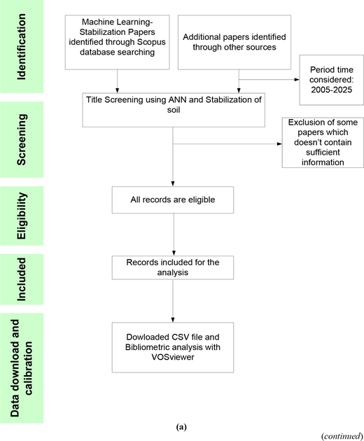
Keyword analysis related to artificial neural network in the area of soil stabilization (a) Prisma flow chart (b) bibliometric analysis using VOSviewer
Source: Author’s own work
Keyword analysis related to artificial neural network in the area of soil stabilization (a) Prisma flow chart (b) bibliometric analysis using VOSviewer
Source: Author’s own work
Studies on the application of ANN in predicting properties of stabilized soil
| Reference | Features | Target | Stabilizing agent/material | No. of data used | Train:test:validation data(%) | Network/training algorithm | No. of input layer neurons | Optimum No. of neurons in hidden layer | No. of output layer neurons | Feature importance/sensitivity analysis | Model performance (testing) | |
|---|---|---|---|---|---|---|---|---|---|---|---|---|
| # | @ | $ | Method * | Result | ||||||||
| Heshmati et al. (2009) | LL, PL, PI, LS, Gr, S, C, L, CC, AC | UCS | CC, L, AC | 219 | 50:25:25 | FFN/RBF | 8 | 32 | 1 | Parametric study | UCS insensitive to LC and CC | R = 0.9667,MSE = 0.071,MAE = 0.188 |
| Alavi et al. (2010) | LL, PI, LS,C, S, L, CC, AC | MDD and OMC | L, CC, AC | 192 | 52:24:24 | MLP/GaA | 9 | 12 (MDD), 10 (OMC) | 1 | Parametric study | G > LL>PI (MDD) G > PI>LS(OMC) | R2 = 0.8916 MSE = 0.895 MAE = 1.13 |
| Das et al. (2011) | LL, PI, C, S, Gr, WC, CC | MDD and OMC | CC | 55 | 67:33:00 | BRNN, LMNN, DENN | 7 | 4 | 1 | GA and CWA | CC > PI>C > LL>S > Gr>WC | MAE = 1.82 AAE = 0.61 RMSE = 0.80 |
| Ouf (2012) | RC, OPC, GGBS, L, CA | UCS and FSP | GGBS, L,RC,OPC | 38 | GeA | 5 | 2 | Min error value < 4% for UCS and <8% for FSP | ||||
| Mozumder and Laskar (2015) | LL, PI, GGBS, FA, MoC, a/B, Na/Al, Si/Al | UCS(28 days) | Geopolymers (GGBS,FA) | 142 | 70:30:00 | MLP/BRNN-BP | 8 | 9 | 1 | GA and CWA | %S>%FA > Na/Al > Si/Al > A/B > MoC>PI > LL | R = 0.982 MSE = 1.50 MAE = 8.34 |
| Sabat (2015) | L, QD, OMC, MDD, CA | CBR (28 days soaked) | L, QD | 90 | 76:24:00 | DENN,LMNN,BRNN | 5 | 5 | 1 | GA | MDD > OMC>L > CA>QD | R2 = 0.981 RMSE = 1.187 MAE = 1.75 AAE = 1.07 |
| Vakili et al. (2015) | P0.005, PI, MDD, L, FC, PoP, CA | Coefficient of permeability (k) | L, pozzolan | 69 | 70:15:15 | MLP/BP | 6 | 9 | 1 | R = 0.99 | ||
| Ayeldeen et al. (2016) | CA, CoE | Gain in strength(%) | CC | 80 | 70:15:15 | FFN/BPA | 2 | 2 layer,8 in each | 1 | R2 = 0.908 | ||
| Belal et al. (2016) | RHA, L, CA, OMC, MDD | CBR (28 days soaked) | L, RHA | 48 | 70:15:15 | FFN/BPA | 5 | 12 | 1 | R = 0.9889 MAE = 0.1644 | ||
| Vinodhkumar and Balaji (2016) | LL, PI, FA, OMC, MDD, NoGl | Soaked CBR | FA, geotextile | LMNN | 6 | 2–30 | 1 | R = 0.9869 MSE = 8.024 × 10⁻¹¹ | ||||
| Ghanizadeh and Rahrovan (2016) | WD cycle, L/SAF, MDD/OMC, σ3, σd | Mr | CKD, FA, FBA | 704 | 60:30:10 | FFN/BPA | 5 | 24 | 1 | R2=0.9857 MSE = 49784(Overall) | ||
| Bahmed et al., 2017 | LL, PL, LC | PI, MDD and OMC | L | 280(PI), 122 (MDD and OMC) | 70:15:15 | LMNN | 3 | 7(PI), 11(MDD), 9(OMC) | 1 | R = 0.9373(PI) R = 0.9356(MDD) R = 0.9406(OMC) | ||
| Salahudeen et al. (2018) | G, LS, FSP, D10, D30, D60, Cu, Cc, LL, PL | MDD and OMC | CKD | 90 | 70:15:15 | MLP/BPA | 10 | 1–10 | 2 | OMC,MDD R = 0.983,9884 MSE = 0.0013,0.001 MAE = 0.0208,0.0321 | ||
| Taha et al. (2018) | C, M, S, G, PI, LL, NM | MDD and OMC | Nano-Cu,Nano-Al,Nano-clay | 75 | 80:20:00 | FFN/BPA | 7 | 1–20 | 1 | Nano clay, Nano Al, Nano-copper(R2=0.987,0.991,0.989) | ||
| Salahudeen and Sadeeq, (2019) | PL, LL, G, LS, Cu, Cc, OMC and MDD | CBR (soaked and unsoaked) | CKD | 72 | 70:15:15 | FFN | 8 | 8(Soaked),17(unsoaked) | 1 | Soaked,Unsoaked R = 0.9986,991 MSE = 0.00013,0.00109 MAE = 0.008,0.012 | ||
| Tinoco et al. (2019) | WC, C, M, S, W/C, CC, OM, CA, CoB, CoSB | UCS | CC | 444 | 70:30:00 | DMA | 10 | 1 | GSA | W/C > CC>OM > CA | R2=0.94 ± 0.001 RMSE = 0.69 ± 0.05 MAE = 0.46 ± 0.02 | |
| Onyelowe et al. (2023) | CC, L, LL, PI, OMC, MDD | UCS | CC,L | 190 | 74:26 | 9 | 5 | 1 | MDD > LL,PL > CC>L > OMC | |||
| Hanandeha et al. (2020) | CC, L, PI, M, C, FA, OMC, WC | Resilient modulus (Mr) | L and FA | 125 | BPA | 8 | 9 | 1 | Parmeteric study by changing input parameter | C > L>FA > PI>C > WC>OMC > M | R2=0.97(training) | |
| Priyadarshee et al. (2020) | C, RHA, CC, PA, CA | UCS | PA,RHA,CC | 129 | 70:15:15 | FFN/LMNN-BP | 5 | 2–11 | 1 | CWA | RHA > PA>C, CC > CA | R = 0.9856 R2=0.9714 MSE = 51.34 RMSE = 7.1651 |
| Rajakumar and Babu (2020) | AsT, AsC, LL, PL, MDD, OMC and NoGeL | Soaked CBR | CoA, BA, GSA and geogrid | 210 | CBLF,GDBLF,LMNN,HWLR | 7 | 7 | 1 | R2=0.97 | |||
| Salahudeen et al. (2020) | G, LS, Cu, Cc, LL, PI, OMC, MDD | UCS(7, 14, 28 days) | CKD | 72 | 70:15:15 | MLP/BPA | 8 | 1–15 | 1 | Soaked,Unsoaked R = 0.99976,9806 MSE = 0.000079,0.000079 | ||
| Shah et al. (2020) | AE, AS, PI, G, OMC, MDD, AASTO, UCS, GI | CBR (10, 30, 65 blows compaction) | Alum sludge waste | 36 | 78:22 | 9 | 1 layer | 3 | 10,30,65 blows R2=0.9892,0.9963,0.9749 RMSE = 0.1586,0.1244,0.5921 | |||
| Hu and Solanki (2021) | 25 properties of cementitiously stabilized subgrade soils. | Mr | CC | RBF,MLP/LM,BRNN,SCG | (Best)25 | 1 and 2 layers(MLP)/(Best)15 neurons | 1 | MSE = 0.5644 (25 - 15-1 layer) | ||||
| Salahudeen et al. (2020) | G, LS, Cu, Cc, LL, PI, OMC, MDD | Durability, Mr, resistance value | CKD | 72 | 70:15:15 | FFN/BPA | 8 | 17(durability),24(resilient modulus),18(resistance value) | 1 | Durability,Mr, resistance R = 0.8388,0.8433,0.7572 MSE = 0.01258,0.01446,0.02368 RMSE = 0.112,0.12,0.154 | ||
| Ngo et al. (2021) | ST, WC, We, CC, CeT D, Sl, Sd, Sa, Sv, ma, De, CA, CuC | UCS | CC | 216 | 80:20:00 | FFN/BPA | 14 | 2–50 | 1 | GB model | We > CC>Ma > WC>De > D>CuC > Sa>Sv > S>CeT > CA>Sd > Sl | UCS 7,14,28 days R = 0.9812,0.9783,0.9942 |
| Tabarsa et al. (2021) | ST, CA, DUW, CC, RHA, L | UCS | CC, L, RHA | 137 | 60:20:20 | MLP/LMNN-BPA | 6 | 7 and 4 | 1 | Statistical software | CC,L > other | R = 0.9957,AAPE = 12.349,AIC = 4.289 |
| Tran (2021) | CC, WC, AF, WFNC | UCS | CC, AF, WFN | 51 | 70:30:00 | LMNN | 4 | 2 layers, 12 and 10 in each | 1 | Relative importance | CC > AF>WC > WFNC | R = 0.94 MAE = 8.6535 RMSE = 10.3390 |
| Pham et al. (2021) | F0.5, F0.25, F0.1, SiO2,Fe2O3,Al2O3,SO3,K2O,CaO,Ti2OCC, CA | UCS | CC | 80 | FFN/LMNN-BPA | 12 | 1 | GA and CWA | CC > F0.5 | R2=0.997 MSE = 0.0415 RMSE = 0.0614 | ||
| Chen et al. (2022) | WC, T, σN, ωt | Shear stress | AGF | 40 | 80:20 | BPNN | 4 | 3 layer, (best-20,20,20) | 1 | Based on BPNN | ωt>σN>T > W | R2=0.948 RMSE = 16.153 MAPE = 24.230 |
| Mustafa et al. (2022) | G, S, M + C, LL, PI, LS,% stabilizer, stabilizer type, OMC, MDD, AR, DW | UCS | Unstabilized, L,CC | 488 | 70:15:15 | LMNN | 12 | 1 layer (24,41,44 for Three dataset) | 1 | Modifying soil chracteristics | R2=0.9883(overall) | |
| Abdallah et al. (2023) | CC, MDD, IWC, CA | UCS, WC and suction | CC | 80:20 | BRBP | 4 | 2 layers, 10 and 5 in each | 3 | UCS, WC, suction R2=0.972,0.932,0.995 | |||
| Aljanabi and Salih (2023) | % of soil, LL, PL, SL, additives(%); additive type | UCS | UIR, UAO, ShP, LGC, WPP, RH, SSP | 74 | 60:20:20, 70:15:15, 80:10:10 | MLP | 6 | 3 layers, 12; (1–7);1 | 1 | Normalized importance | Additive type > additives(%); >PL > LL> SL>% of soil | R = 0.98 |
| Krishna et al. (2023) | LL, PL, OMC, MDD, L, CC, FA (for UCS) & UCS (for CBR) | CBR and UCS | L, CC, FA | 125 | 80:10:10 | FFN/LMNN-BPA | 7(UCS)&8(CBR) | 2 layer, 10 in each | 1 | CBR,UCS R2=0.924,0.95 MAE = 0.45228,0.0166 RMSE = 0.00537,0.0012 | ||
| Kumar et al. (2023) | Soil(%), CC, L, LL, PL, PI, MDD, OMC | UCS | L,CC | 100 | 60:10:30 | LMNN-BP | 8 | 2 layer, 16 and 32 neurons each(best) | 1 | R = 0.70 | ||
| Lu et al., 2023 | S, M, C, LI, Wc/Cc | UCS | CC | 80 | 80:20 | LM, BR | 5 | 1,2,3,4,5 layers and 60 neurons | 1 | Varying value of input parameter | Wc/Cc > M > S > C>LI | R2=0.896 MSE = 13667.232 RMSE = 116.907 MAE = 102.584 MSLE = 0.042 RMSLE = 0.206 |
| Onyelowe et al. (2024) | WGP, NACL, PA, LL, PL, FSI, OMC, MDD | CBR,UCS | WGP,NACL,PA | 25 | 80:20 | BPNN | 8 | 1 layer (1,2,3 neurons) | 2 | Relative importance | OMC > WGP>PA > NACL>FSI > LL>PL > MDD | CBR,UCS SSE = 1.5%,2% R2=0.9979,0.9973 |
| Anh et al. (2024) | WC, LL, PL, Wab | Aps | PSAS | 147 | 60:20:20 | MLP/BP ANN and GA ANN | 4 | 2–12-BP ANN, 8-GA ANN | 1 | BP, GA R2=0.9269,0.9121 MSE = 0.0299,0.0244 | ||
| Baldovino et al. (2024) | CA, MDD, WGP(%), CC, VWC, VCC, WGP + CC, P/CCi,P/Bi | UCS(7 and 28 days), Stiffness | WGP, CC | 72 | 70:15:15 | BP | 1 layer,9 | 1 | Stiffness, UCS R2=1,1 RMSE = 0.0384,0.0021 | |||
| Goutham and Krishnaiah (2024) | BA, L, LL, PL, SL, MDD, OMC | UCS(28 days) | BA, L | 79 | 70:30 | MLP/LMNN-BPA | 7 | 7 | 1 | GA and CWA | LL > L>SL > BA>PL > MDD > OMC (GaA), BA > OMC>MDD > SL>LL > L>PL (CWA) | R2=0.99 |
| Mojtahedi et al. (2024) | CA, W/C, CC, PI, G, S, C | UCS by deep mixing | CC | 192 | 75:25 | FFBP | 7 | 1 layer, 7 &12 | 1 | Analyzing current weights | G > W/CC > C > S > CA>CC > PI | R2=0.992 |
| Thapa et al. (2024) | C,M, NS, BC, SI, MDD, WC, omc | CBR | NS, BC | 175 | LMNN-BPA | 6 | 1layer, 10 neurons | 1 | XAI (SHAP and LIME) | C > M>MC > NS/BC > SI>MDD | R2=0.958 MSE = 0.02 RMSE = 0.049 MAE = 0.085 | |
| Wani and Thagunna (2024) | GSD, PI, LL, PL, WC, FA, CA | Shear strength | FA | 85:15 | 7 | 5 layer | 1 | FA > CA>other | R2=0.69 MSE = 0.01 | |||
| Mohammed et al. (2025) | CA, MDD, OMC, GGBS, PL, LL, PI | UCS | GGBS | 200 | 80:20 | 7 | 1 | SHAP and LIME | CA > OMC>MDD > GGBS>PL > LL>PI (SHAP) | R2=0.94 RMSE = 0.15 MAE = 0.037 | ||
| Sharma et al. (2024) | L, CA, PI, pH, Vp, OMC, MDD | UCS, E, c, ϕ | L | 54 | 80:20 | 7 | 10 | 4 | UCS,E,c,ϕ R2=0.887,0.926,0.805,0.859 RMSE = 20.984,3.654,6.019,2.338 MAPE-7.722,13.338,10.325,6.803 | |||
# LL= Liquid Limit, PL= Plastic Limit, SL=Shrikage Limit, PI=Plasticity Index, C= clay content, M= silt content, S= sand content, Gr=gravel content, G=Specific gravity, WC=Water content, CC=Cement Content, CA=Curing age/time, LS=linear shrinkage, L=Lime, AC=Asphalt content, RC=Road Cement, OPC=Ordinary Portland cement, GGBS=Ground Granulated Blast Furnace Slag, FA=Fly ash, MoC=Molar concentration, A/B=Alkali to binder ratio, Na/Al=atomic ratio of sodium to aluminate, Si/Al=atomic ratio of silicate to aluminate, QD=Quarry dust, MDD=maximum dry density, OMC=optimum moisture content, P0.005=Percentage finer than 0.005 mm, PoP=Pozzolon percentage, FC=fine content, CoE=Compaction energy, RHA=Rice husk ash, NoGl=Number of geotextile layer, G= specific gravity, grain sizes -(D10,D30,D60), Cu-uniformity coefficient, Cc-coefficient of curvature, Water/cement ratio=W/C, OM=Soil organic matter, Coefficient related with the binder type=CoB, Coefficient related with a secondary binder=CoSB, PA-Pond ash, OM=organic matter content, ST=Soil type, We=Wet density, CeT-Cement type, D-Soil sampling depth, Sl=specimen length, Sd=specimen diameter, Sa=specimen area, Sv=specimen volume, Ms=Mass of specimen, De=Density of specimen, CA, CuC=Curing condition, AsT=Ash type, AsC=Ash content, NoGel=Number of Geogrid layers, AF=Air foam, WFNC= Waste fishing net content, F0.5,F0.25,F0.1=Particle size distribution, SiO2,Fe2O3,Al2O3,SO3,K2O,CaO,Ti2O=Chemical composition, WD cycle=Wetting and Drying cycle, L/SAF=ratio of Free Lime to Silica, Alumina and Ferric Oxide compounds in the cementitious materials, MDD/OMC=ratio of maximum dry density to the optimum moisture content, σ3=confining stress, σd=deviator stress, BA=Bagasse ash, NM=Nano Material, DUW=dry unit weight, WGP=Waste glass powder, VGW=volumetric water content, VCC= volumetric cement content, WGP + CC=volumetric content of the sum of WGP and cement, P/Ci=porosity/cement index, P/Bi=porosity/binder index, IWC=Initial water content, LI=Liquidity Index, Wc/Cc = Water content/Cement content, Vp=primary ultrasonic wave velocity, pH=potential of hydrogen, T =Temperature, σN=Normal stress, ωt= Shear displacement, AR=Aspect ratio, DW=Testing condition, GSD=Grain size distribution, AE=Applied energy, AS=Alum sludge, AASHTO =American Association of state highway and transportation, GI=Group index, NACL=Sodium Chloride content, FSI=Free swell Index, NS=Nano-silica, BC=Bio-char, SI=Soil index
@ OMC = optimum moisture content; MDD = maximum dry density; UCS = Unconfined compressive strength; CBR = California bearing ratio; Mr = Resilient Modulus, Aps = Amount of paper sludge ash stabilizer
! MSE = Mean squared error; MSLE = Mean squared logarithmic error; RMSE = Root mean squared error; RMSLE = Root mean squared logarithmic; E = modulus of elasticity; c = cohesion; Φ = angle of internal friction
$- CC = Cement Content, L = Lime, AC = Asphalt content, RC = Road Cement, OPC = Ordinary Portland cement, GGBS = Ground Granulated Blast Furnace Slag, QD = Quarry dust, PoP = Pozzolon percentage, FA = Fly ash, CKD-Cement klin dust, PA=Pond ash, RHA = Rice husk ash, CoA = Coal ash, BA = Bagasse ash, GSA = Groundnut shell ash, PSAS = Paper sludge ash stabilizer, FBA = Fluidized bed ash, UIR = iron ore, UAO = used automobile oil, ShP-shale rock powder, LGC = a mixture of hydrated lime, gypsum and cement, WPP = waste plastic pieces, RH = rice husk, SSP = sandstone powder, AGF = Artificial ground freezing
c FFN=Feed forward network, RBF=Radial Basis Function MLP=Multi-layer perceptron, BP=Backpropagation, BPA=Back propagation algorithm, GaA=Garson Algorithm, BRNN=Bayesian regularization method, LMN=Levenberg-Marquardt algorithm, DENN=differential evolution algorithm, GeA=General algorithm, DMA=Data Mining algorithm, CBLF=Conscience bias Learning function, GDBLF=Gradient descent weight and Bias learning function, HWLR=Hebb weight learning rule, RBF=Radial Bias Function, SCG=Scaled conjugate gradient, ABC-ANN=artificial bee colony-ANN hybrid
* GA = Garson Algorithm, CWA = Connection weight approach, GSA = Global sensitivity analysis, GB = Gradient boosting, BR = Bayesian Regularization, BRBP = Bayesian Regularization backpropogation, SHAP = Shapely Additive Explanation, LIME = Local Interpretable Model-agnostic Explanations, XAI = Explainable Artificial Intelligence
> indicates superior
Each tested model’s performance is assessed by calculating errors using specific loss functions as given in Table 1. Common loss functions include the mean squared error (MSE), mean absolute error (MAE), root mean squared error (RMSE) and the coefficient of determination (R2), along with others. Vinodhkumar and Balaji (2016) suggested that an ANN model can be evaluated using the Regression R-value (or Coefficient of determination, R2 value) and the MSE. These metrics can be computed using equations (3) to (6).
Coefficient of determination (R2): Assesses the quality of predictions in a regression model. The regression R2 value measures the correlation between the predicted outputs and the actual targets (shown in equation (1)), with an R2 value of 1 representing a perfect relationship and a value of 0 indicating no correlation between the variables:
Mean Square Error (MSE): It quantifies the average of the squared differences between actual and predicted values, ensuring that the predicted value is as close as possible to the actual outcomes. A lower MSE denotes improved prediction accuracy, with zero indicating no error. It is expressed as per equation (2):
Root mean square error (RMSE): Often preferred over MSE as it provides a more interpretable measure of error:
Mean Absolute Error (MAE): It reflects the average deviation between predicted and actual values, serving as an indicator of the model’s predictive accuracy:
where yi is the actual target value, n is the number of observations, y the mean value of the actual target, ŷi is the predicted output value and Var is the variance of the target variable(y).
4.1 Target variables of stabilized soils using artificial neural network
As summarized in Table 1, attempts have been made to forecast the stabilized soil properties that uses stabilizers like cement, lime (Ground granulated blast furnace slag, GGBS), fly ash, rice husk ash, pond ash, fiber content, geogrid and geopolymers using ANN. The ANN models were used to predict parameters such as OMC, UCS, MDD, CBR, permeability, resilient modulus, durability, resistance value, free swell potential (FSP) and Brazilian tensile strength (BTS). Alavi et al. (2010) developed separate ANN models to predict the OMC and MDD, along with a combined model capable of simultaneously estimating both parameters (multiple outputs). Several subsequent studies have also incorporated multiple soil property outputs to evaluate the characteristics of stabilized soils (Ouf, 2012; Salahudeen et al., 2018; Shah et al., 2020; Abdallah et al., 2023; Onyelowe et al., 2024; Sharma et al., 2024).
The conventional approach to constructing flexible pavements on soft soil includes forming a more rigid, load-bearing base over the soft subgrade. The necessary thickness of this base is calculated based on the subgrade’s desired CBR value and/or UCS value. However, the required base thickness can become substantial when dealing with very soft to soft subgrades, such as black clays which are characterized by a high swelling content. In such cases, using chemical modification can significantly reduce the needed base thickness compared to other modification techniques. Additionally, chemical stabilization enhances the performance of the geotechnical structure by preventing the base material from migrating into the subgrade (Salahudeen et al., 2020).
The unconfined compressive strength test is commonly used to find durability and resistance values. Durability, defined as the capacity to maintain stability and integrity under prolonged exposure to adverse environmental conditions, is a key factor in additive-based stabilized soil layers for pavement design. For a pavement layer, preserving its properties throughout its lifespan is essential. Climatic variations are a significant factor affecting pavement performance. The resistance value, which indicates a material’s resistance to strength loss under adverse field conditions, is an important property, particularly in pavement construction. It evaluates the material’s ability to retain strength while submerged in water. Vertical loading on foundation materials frequently leads to lateral deformation, with the resistance value indicating the material’s ability to endure this failure mode. This value is obtained by evaluating the soil specimen’s resistance to strength loss (Salahudeen et al., 2022). The Brazilian tensile strength (BTS) test is conducted in the laboratory to determine the tensile strength of brittle materials like unsaturated soils. It is essential for assessing rock tensile strength and soil mechanical properties. To consider the geotechnical aspect, it is important in projects like slope stability and bearing capacity.
The California Bearing Ratio (CBR) serves as an indicator of subgrade soil strength. A representative sample is collected, and a remolded specimen is prepared to conduct a CBR test on the soil. This specimen is compacted at the predetermined optimum moisture content (OMC) using modified Proctor (light) compaction. The prepared specimen is then soaked in water for few days before conducting the penetration test. The soaked CBR value of a soil sample is typically obtained in about a week (Rajakumar and Babu, 2020). When the CBR value of soil is low, a thicker pavement is required, which increases construction costs, and conversely, a higher CBR value reduces both thickness and cost (Sabat, 2013). Resilient modulus is another significant parameter in pavement design, measuring a material’s elastic modulus under a given stress. Thus, accurately measuring the resilient modulus is crucial for ensuring the efficiency and precision of the design of pavement. It is defined as the ratio of the applied deviator stress to the recoverable strain and represents the material strength of the pavement layers. The resilient modulus values were determined through cyclic load tests (repeated load triaxial test) following AASHTO T307 standards. Salahudeen et al. (2022) and Ghanizadeh and Rahrovan (2016) used ANN for predicting the resilient modulus of treated soil.
For applications like earth embankments and dam designs, understanding soil permeability is crucial. The falling head test is a common method for evaluating the permeability of fine-grained soil (Erzin et al., 2009). Understanding index properties like OMC and MDD is essential for both field and laboratory soil compaction processes. OMC represents the water content at which the MDD is attained (Salahudeen et al., 2018). Free swell potential (FSP) refers to the volume increase of soil when submerged in water without any external pressure (Chen, 2012). It aids in identifying the potential of soil to swell.
All the tests mentioned above, however, are time-intensive, demand skilled personnel and require costly laboratory equipment. As an alternative, these parameters can be accurately predicted using ANN simulations. This is achievable because the parameters are linked to various soil index properties. The UCS and CBR values, critical in pavement design, can be forecasted using ANN, which is particularly relevant in geotechnical investigations aiming to enhance soil stability (Krishna et al., 2023). Many studies are available to predict index properties like OMC and MDD of stabilized soil using ANN (Alavi et al., 2010; Das et al., 2011). However, only limited studies are available to determine parameters like BTS (Chore and Magar, 2017), Resilient modulus (Salahudeen et al., 2022), permeability (Vakili et al., 2015) and FSP (Ouf, 2012) that have been successfully modeled using ANN. All the above-mentioned parameters serve as target variables in ANN modeling efforts.
4.2 Independent variables for prediction of stabilized soil properties using ANN
In soil stabilization problems using ML, the inputs can be mentioned as independent variables. Critical input parameters for ANN-based prediction of stabilized soil properties, typically include index properties such as specific gravity (GS), plastic limit (wp), liquid limit (wL), plasticity index (IP), grain size, coefficient of curvature (Cc), uniformity coefficient (Cu), linear shrinkage (LS), percentage of stabilizer, curing time (CT) and compaction duration as seen in Table 1. The input parameters influenced by the target variable may vary. For instance, Kalkan et al. (2009) highlighted that the UCS values of stabilized soil are influenced by several factors, including the water content in compacted soil, soil particle composition (gravel, sand, silt and clay contents), compaction effort, as well as the shape and size of the particles. In contrast, Pham et al. (2021) emphasized that UCS values primarily depend on factors such as stabilizer content, chemical composition, water content and curing time. Lorenzo and Bergado (2004) concluded from their study that the post-stabilization behavior of soil is generally influenced by independent variables like soil type, water content, plasticity, compaction characteristics, type and percentage of stabilizer and curing time. Mozumder and Laskar (2015) have considered some properties of additives like alkaline activator molarity, the sodium-to-aluminium ratio and silicon-to-aluminium ratio in the activator binder mixture as the input parameter along with wL, wp, GGBS and FA content.
It is essential to note that some soil property variables are inherently interdependent, i.e. transformation uncertain. This interdependency can complicate analysis by exaggerating the relationships between variables. Gravel content, for instance, is calculated by subtracting the combined percentages of sand and clay/silt from 100, while the plastic limit is determined by subtracting the plasticity index from the liquid limit. Consequently, both gravel content and the plastic limit are excluded as input variables in the ANN model. However, clay/silt, sand, plasticity index and liquid limit, are mostly retained despite their potential redundancy, owing to their traditional relevance as soil condition indicators and their advantageous value distributions (Heshmati et al., 2009; Alavi et al., 2010).
Stabilization methods aim to determine the best combination of stabilizing agents through extensive data analysis, often requiring RA to establish relationships between variables and develop necessary models (Jeremiah et al., 2021). Consequently, the significant variability of factors increases the complexity of the analysis. Although many studies have concentrated on limited parameter sets and used simplified mathematical models, ANNs provide a more robust alternative. By enabling the simultaneous analysis of multiple dependent and independent variables within a single experimental data set, ANNs uncover intricate, non-linear relationships that often elude traditional regression techniques. Principal Component Analysis (PCA) can be applied before training the ANN model to transform and reduce the number of input features (Abdallah et al., 2023). By doing so, it removes redundant or highly correlated variables, captures the most important patterns in the data and simplifies the input space. This helps the ANN learn more efficiently, avoid overfitting and ultimately improve the model’s predictive accuracy and performance. Abdallah et al. (2023) suggested that to mitigate overfitting, the training process can be terminated at the point where the MSE on the testing data set attained its minimum value.
4.3 Analytical process for forecasting stabilized soil characteristics via ANN
The processes for analyzing and predicting the properties of stabilized soil with ANN are depicted in Figure 4. A comprehensive explanation is outlined as follows.
 The workflow diagram shows a process beginning with data collection followed by data preprocessing. The dataset is separated into training data and testing data and proceeds to feature scaling. The prepared data are used for model training and testing using feed forward and recurrent neural network models. Model optimization and evaluation follow the training stage. Model validation includes evaluation metrics M S E, R M S E, M A E, and R 2. The workflow ends with selection of the optimum model.
Process of analysis using ANN for the prediction of stabilized soil properties
Source: Author’s own work
The workflow diagram shows a process beginning with data collection followed by data preprocessing. The dataset is separated into training data and testing data and proceeds to feature scaling. The prepared data are used for model training and testing using feed forward and recurrent neural network models. Model optimization and evaluation follow the training stage. Model validation includes evaluation metrics M S E, R M S E, M A E, and R 2. The workflow ends with selection of the optimum model.Process of analysis using ANN for the prediction of stabilized soil properties
Source: Author’s own work
4.3.1 Data collection
For predicting the properties using ANN, the required data has to be collected. The analysis process commences with data collection, achieved through experimental analysis or by accessing databases such as Scopus, ScienceDirect and Web of Science to gather unbiased experimental data. If the data is collected from experimental studies, then initially, the soil and the additives used in the study were characterized according to standards like Indian standards, American Society of Testing Material (ASTM) standards or British standards (Belal et al., 2016; Salahudeen and Sadeeq, 2019). The stabilization of the soil has to be performed with the additive. The intended post-stabilization behavior of soil like UCS, MDD, OMC, CBR, Resilient modulus or permeability values has to be determined. Some test, like the CBR test, was performed on 0, 7 and 28-day cured samples (Belal et al., 2016).
This collected data, organized for a specific problem, is referred to as a data set. In some cases, as seen in Table 1, models were developed using data from single experimental studies, which may restrict their relevance to engineering applications. The effectiveness of an ANN is heavily dependent on the accuracy and volume of data available in its database (Bahmed et al., 2017). Data sets are tailored to different purposes and are typically stored in formats like CSV, HTML or XLSX files for use in coding.
4.3.2 Data preparation and preprocessing
Data preparation and preprocessing involve converting raw data into an appropriate format for a machine-learning model. Initially, the collected data undergoes preprocessing to ensure consistency for data analysis. Experimental data’s descriptive statistics, obtained through various laboratory tests, served as the foundation for developing the ANN model (Salahudeen et al., 2018). It includes determining minimum, maximum, standard deviation, mean, coefficient of variation (CoV), kurtosis and skewness, which are performed on the entire data set. Missing value, outlier and duplicate treatment can also be performed in the process of data preprocessing. The range of data used for the analysis using ANN from the previous studies is around 28–704 No’s as shown in Table 1.
The preprocessed data is typically divided into testing, training and validation sets in specific proportions. The training set establishes relationships between dependent and independent variables, while the test set evaluates model performance. The learning process was terminated using a validation set (Bahmed et al., 2017). The key idea is to monitor the validation loss (or other validation metrics, such as accuracy or error) after each epoch (iteration through the training data). If the validation loss keeps decreasing, it means the model is continuing to improve. However, if the validation loss starts increasing, it specifies that the model is beginning to overfit the training data, meaning it’s learning noise or irrelevant patterns that don’t generalize well to new data. In data preprocessing, the data set is often divided into various proportions for training, testing and validation, such as 70:15:15 (Vakili et al., 2015; Ayeldeen et al., 2016), 70:30 (Sabat, 2015), 80:20 (Ngo et al., 2021) and 52:24:24 (Alavi et al., 2010) and 80:10:10 (Krishna et al., 2023) as shown in Table 1. Normally, the training set comprises 70% to 80% of the data, with the remaining 20% to 30% used for testing. Within the test set, some percentage may be reserved for validation (Belal et al., 2016; Salahudeen and Sadeeq, 2019; Vakili et al., 2015). This approach enables the model to train on a significant portion of the data set while assessing its performance on unobserved data.
4.3.3 Feature scaling
Once the database is divided, data should be normalized before being introduced to the ANN models to maintain consistency within the limits of the activation/transfer function applied to both the output and hidden layers (Bahmed et al., 2017). Normalization can be performed using various standardization methods such as the Z-score method (Zhang et al., 2023), the min-max normalization method (Jeremiah et al., 2021) and median and MAD (Median Absolute Deviation), tanh estimators. The Z-score method measures how far a data point deviates from the mean in terms of standard deviations, transforming data to have a mean of 0 and a standard deviation of 1. It is effective when data follow a normal distribution and helps stabilize the training process of most ML models. The min-max normalization rescales data to a fixed range, usually [0, 1] or [−1, 1], preserving the relationships among original values while eliminating scale differences across variables. It is particularly useful for neural networks and gradient-based optimization methods where feature magnitude influences learning. Median and MAD normalization is robust to outliers and is preferable for data sets with skewed distributions or extreme values. Tanh estimators provide a nonlinear scaling that limits the impact of outliers while maintaining smooth gradients, which can improve convergence stability in certain ML applications. In general, the best normalization method depends on the data set characteristics and the learning algorithm. For neural network models, min-max normalization is most commonly used and typically yields the best performance due to its compatibility with activation functions (e.g. sigmoid, tanh and ReLU). For data sets with outliers, Z-score or median–MAD methods may produce more reliable results.
Both Mozumder and Laskar (2015) and Salahudeen et al. (2018) divided the available data into subsets, with input and output data normalized between −1 and 1. The tangent sigmoid function’s output remains within this specified range. While sigmoid functions are typically used as the transfer function for each node in stabilized soil analysis (Erzin et al., 2009), alternatives like linear and hyperbolic tangent functions can also be used, depending on the variable characteristics (Vakili et al., 2015). To avoid saturation in the data set, Priyadarshee et al. (2020) selected a range of [0.1, 0.9]. However, it is generally advised to normalize the inputs to the range of [−1, + 1], as this has been proven to improve learning speed significantly (Alavi et al., 2010; Das et al., 2011). This ensures that input values lie within the optimal region of the sigmoid transfer function, where output sensitivity to input variations is maximized. The normalized data is then fed into the neural network, where individual weights are assigned to the variables and visualized during the training process.
4.3.4 Model training and testing
This section primarily describes the network architecture and the important hyperparameters that govern the training and performance of the ANN model. The hyperparameters used in ANN define the structure of the network and influence the training process significantly. Some of the key hyperparameters and components include the network type, training algorithm, transfer function, activation function, performance function, training epochs, learning rate, number of inputs, output and hidden layers and number of neurons in each layer. These factors are important because they define the model’s capacity, determine how well it will fit the training data, and generalize to new, unseen data. Proper tuning of these parameters is crucial for achieving optimal performance.
Developing an initial model necessitates careful consideration. Network type specifies the architecture of the network (e.g. convolutional neural network, fully connected feedforward neural network, recurrent neural network). Training algorithm refers to the method used for training the network, which often involves an optimization algorithm like Gradient Descent, Adam and RMSprop to minimize the loss function. Sabat (2015) postulated that ANN models for stabilized soil properties can be developed using different training algorithms such as Bayesian Regularization (BR), Differential Evolution (DE) and Levenberg–Marquardt (LM) to establish regression models. Levengberg–Marquardt (LM) algorithm was proven to be the fastest training algorithm for multilayer perception and is particularly effective in expediting convergence during model training for stabilization problems (Vinodhkumar and Balaji, 2016; Bahmed et al., 2017; Jeremiah et al., 2021). This algorithm also has the ability to minimize error and achieve the highest R2 values (Sabat, 2015). LM algorithm produces a solution called least squares.
The ANN models can use learning functions like gradient descent weight and bias learning, conscience bias learning, Hebb weight learning rule, gradient descent with momentum weight (Rajakumar and Babu, 2020) and various backpropagation methods, including conjugate gradient with Powell-Beale restarts, Quasi-Newton, scaled conjugate gradient, Fletcher–Reeves updates and Polak-Ribiére updates (Vinodhkumar and Balaji, 2016). Jeremiah et al. (2021) studied post-stabilization behavior of treated clays using lime, geopolymers and cementitious by-products, with particular emphasis on the application of backpropagation ANN models. The various networks and algorithms used for the prediction of stabilized soil properties are shown in Table 1. From Table 1, the most common network used for predicting stabilized soil properties includes the feed-forward network, and the algorithms used include the Levenberg–Marquardt and BPAs. LM algorithm can be combined with the BPA to train ANNs. For example, the LM algorithm can be used to adjust the bias and weight variables. In contrast, the BPA can be used to estimate the Jacobian matrix of the performance function.
The activation function {f ()} introduces non-linearities into the network and is selected according to the specific needs of the problem the neuron is addressing. There are various types of activation functions, including sigmoid, commonly used for non-linear problems, and linear function, often used for linear problems (Krishna et al., 2023). The sigmoid types include (a) Hyperbolic tan-sigmoid (Tanh) (Sabat, 2015) and (b) Log-sigmoid (Logistic) (Vakili et al., 2015). ReLU (Rectified Linear Unit) is another most frequently used activation function in ANN, especially in hidden layers. Even two types of transfer functions can be used in one ANN network. For instance, the purely linear function for the output layer and the tanh (hyperbolic tangent) function for the hidden layer to generate the output of the processing element (Salahudeen et al., 2018). The transformed output from hidden layers serves as the input to the output nodes in the output layer, where further processing occurs to determine the predicted value.
Training epochs refer to the total number of times the training data set is passed through the model or the maximum number of iterations the training process will run. An epoch involves one forward and one backward pass of all training examples. The learning rate is a key hyperparameter that governs the size of the steps the optimizer takes when adjusting the model weights. Too high a learning rate can lead to instability, while too low a rate can make the learning process too slow. From the works of literature reviewed, the maximum iteration (epochs) can range from 1,000 to 5,000, and the Learning rate ranges from 0.00001 to 0.2.
The input layer in an ANN generally includes neurons corresponding to the number of input variables (Priyadarshee et al., 2020). During training, selecting the optimal configuration of the hidden layer is essential, as an arbitrary choice of hidden neurons may result in overfitting or underfitting problems (Gnana Sheela and Deepa, 2013). From Table 1, for the prediction of stabilized soil properties, the hidden layers commonly consist of one or two layers. In their study, Salahudeen et al. (2018) applied separate ANN models, using five neurons for predicting OMC and seven neurons for MDD. The choice of an appropriate number of neurons in the hidden layer plays a crucial role, as too many layers or neurons can lead to longer analysis durations and overfitting risks (Jeremiah et al., 2021). To enhance the performance of the ANN model, the number of neurons in the hidden layer can be optimized using a trial-and-error approach (Belal et al., 2016; Priyadarshee et al., 2020). While no universal rules exist for determining the number of hidden layers or neurons per layer, a simple architecture such as a single hidden layer with a limited number of neurons is generally recommended during the learning phase (Bahmed et al., 2017). One common guideline suggests using the average of neurons in the output and input layers (Alavi et al., 2010), while another proposes allocating 60–70% of the total neurons from these layers to the hidden layer. For instance, Belal et al. (2016) identified an optimal configuration with one hidden layer containing 12 neurons, based on performance metrics like the mean absolute error (MAE) and correlation coefficient (R2). Their model demonstrated low MAE and high R2 values, indicating robust performance on the training data.
In many stabilization-related ANN analyses, a single hidden layer has demonstrated effectiveness. The hidden layer neurons can better be selected based on the objective of establishing a reasonable starting point for optimization during training, adjusting weights based on performance metrics such as, RMSE, MSE, mean average error (MAE) and correlation coefficient (R2). The output layer typically comprises one or more neurons depending on the number of desired outputs. Salahudeen and Sadeeq (2019) selected different ANN models to determine the soaked and Unsoaked CBR values. The close proximity between predicted and experimental values underscored the accuracy of the predictive model developed. Thus, ANN training algorithms can be used with varying numbers of hidden layer neurons to identify the best model structure.
The model training in ANN determines the weights, which is similar to identifying the polynomial coefficients in RA (Ayeldeen et al., 2016). The capacity of a multilayer neural network to learn from examples is based on the activation and interconnection models, where the information is stored in the weights of the connections (Bahmed et al., 2017). Model training involves adjusting hyperparameters like weights and biases to minimize a loss function (Hamed et al., 2004; Kalantary and Kordnaeij, 2012). Initially, weights are assigned randomly, and an iterative algorithm is used to find the optimal weights that lessen the variance between the predicted and actual outputs (Nasr et al., 2013). Hyperparameters can be iteratively fine-tuned to achieve an optimal model using methods such as grid search (GS) and random search (RS) or advanced global optimization techniques like GAs, Bayesian optimization and particle swarm optimization. These methods help to identify the best combination of hyperparameters to improve the model’s performance effectively. Ngo et al. (2021) suggested that among those algorithms, GS and RS showed simple algorithms and good performance as these have different strategies for searching in hyperparameters space. Anh et al. (2024) suggested GA-ANN converges faster compared to the commonly used BPA, BP-ANN, hence able to predict with higher accuracy and within a shorter period.
4.3.5 Model optimization and evaluation
In ANNs, optimization algorithms (often referred to as solvers) are critical for updating the model’s weights during the training process. By using the gradients of the loss function, these solvers iteratively modify the weights to minimize the loss and optimize the model’s performance. The commonly used solvers in ANN include the Stochastic Gradient Descent, the Quasi-Newton method and Adam (Ngo et al., 2021).
Jeremiah et al. (2021) recommend using a training data set size of at least ten times the number of network parameters given. With a limited training data set, the model’s capacity to apply to unseen data may be impaired by overfitting, a common issue encountered in ANN applications for soil stabilization research (Belal et al., 2016). Using methods like cross-validation (CV) and bootstrapping, models are trained on diverse subsets of the training data set to estimate their effectiveness on unfamiliar, untested data. CV, a common resampling procedure, evaluates ML models on a limited data sample to predict their general performance beyond the training data. It is preferred for providing a less biased estimate compared to a simple train/test split, thereby reducing the model’s reliance on the initial data split and minimizing variance in performance metrics. Different CV techniques are available, with K-fold CV being especially suitable for small data sets. K-fold CV is extensively used in ML for model training and evaluation, helping to mitigate overfitting in the final model (Ngo et al., 2021). In K-fold CV, the training data set is divided into K subsets and the model is trained and validated iteratively across K folds. Every iteration uses K-1 folds for training and one fold for validation, with the overall performance averaged across all iterations (Ngo et al., 2021). The model can be refined multiple times; for instance, in 10-fold CV, the model is trained and validated across ten iterations, enhancing generalization capability (Huo et al., 2022; Zhang et al., 2023). Leave-one-out CV represents an extreme case where each data point serves as a test set once. However, in the majority of the reviewed studies on stabilized soil properties, ANN models were validated using basic train-test splits rather than CV. Incorporating K-fold or LOOCV in future research is recommended to improve model reliability and ensure robust predictive performance, particularly for data sets of limited size.
Bootstrapping is another method used to evaluate the quality of ML models. It involves generating results for a population by repeatedly sampling smaller random subsets (with replacement) from the population. Subsequently, fitting the data often involves using ensemble methods such as bagging and boosting. In bagging, multiple models are trained separately and their predictions are combined using methods such as voting or averaging. In contrast, boosting builds models sequentially, with each subsequent model focusing on correcting the errors of its predecessor, resulting in a more robust ensemble.
Following the training process, the model’s performance is analyzed using a data set that has not been previously encountered. This evaluation involves an iterative process of model training and validation, where hyperparameters are adjusted until the optimal results are achieved (Taffese and Abegaz, 2021). Model performance is typically evaluated using loss functions (Salahudeen et al., 2020) and the architecture was fine-tuned by testing varying numbers of neurons in the hidden layer, generally ranging from 1 to 20. Metrics such as MSE and R2 values were used for assessment (Salahudeen and Sadeeq, 2019). Once the output is predicted, it should be compared to the corresponding actual value to evaluate the performance of the ANN and verify the accuracy of the developed model.
The common loss functions and the equations for finding those functions were explained previously. These metrics collectively offer a comprehensive approach to model performance across various fields. Optimally, the coefficient of determination and correlation coefficient should be high, while MSE, RMSE and MAE should be minimized. When outcomes fall short, backward propagation adjusts weight values to optimize the loss function, iteratively refined through an optimization algorithm implementing backpropagation. The entire process is iterative, continuing until the loss functions are minimized. During each training procedure, adjustments are made to the hyperparameters like transfer function, training algorithm and initial weight assignments until identifying the network architecture that delivers the most favorable outcomes (Kalkan et al., 2009). If both the training and validation results show satisfactory performance, the model can be considered reliable for making predictions. In the case of ANNs, overfitting usually occurs when the error in the training phase is lower than that in the validation phase (Baldovino et al., 2024).
4.3.6 Sensitivity analysis/selection of important input variable
Sensitivity analysis is used to quantify the impact of different input parameters. It was performed to evaluate the extent of each variable’s contribution to the model’s predictions (Pham et al., 2021). Due to their complex and nontransparent structure, ANNs are frequently described as “black boxes,” making it difficult to anticipate the process by which models are selected (Das et al., 2011). Nevertheless, sensitivity analysis can shed light on the impact of input variables on the target variable (Das et al., 2011; Ngo et al., 2021; Jeremiah et al., 2021). Alavi et al. (2010) and Das et al. (2011) applied the Garson algorithm (Garson, 1991) to evaluate the contribution of individual input variables in the ANN model for predicting the OMC and MDD of stabilized soil. Sabat (2015) used the Garson algorithm for sensitivity analysis to identify key input variables for forecasting the CBR values of soil stabilized using quarry dust and lime. According to his findings, MDD and OMC are crucial parameters for predicting the CBR value of stabilized soil. They found that textural properties like clay and sand content and plasticity characteristics such as liquid limit and plasticity index were more important than other variables like percentage of stabilizers and linear shrinkage. From their research, Mozumder and Laskar (2015) indicated that the connection weight approach is superior to Garson’s algorithm in recognizing the actual relevance of input variables in UCS prediction. They noted that both approaches placed the percentage of sand as the most influential parameter, whereas PI and LL were regarded as the least significant. To generate simplified interpretations of complex ML models, recent studies (Thapa et al., 2024; Mohammed et al., 2025) have used explainable artificial intelligence (XAI) approaches, including Shapley Additive Explanations (SHAP) and Local Interpretable Model-Agnostic Explanations (LIME). Table 1 includes the result of the sensitivity analysis performed while determining the stabilized soil properties using ANN. A neural interpretation diagram (NID) can be used to interpret connection weights among neurons visually. The approach is used to illustrate the connection between input variables and the resulting output. Figure 5 illustrates a typical Neural Interaction Diagram (NID) based on data from Sabat (2015), where the thickness of the lines represents the relative strength of the connection weights. It was found from their study that the quarry dust (QD) and curing age (CA) indicated as grey circles specify the least influential parameters for predicting the CBR value, while percentage of lime (L), OMC and MDD in black circles represent more influential parameters. It visually represents the input’s influence on the output.
 The neural network architecture diagram shows five input neurons labeled Q D, C A, L, O M C, and M D D connected to a layer of hidden neurons through multiple weighted connections. The hidden neurons connect to a single output neuron labeled C B R.
Typical neural interpretation diagram
Source: Author’s own work
The neural network architecture diagram shows five input neurons labeled Q D, C A, L, O M C, and M D D connected to a layer of hidden neurons through multiple weighted connections. The hidden neurons connect to a single output neuron labeled C B R.Typical neural interpretation diagram
Source: Author’s own work
5. Limitation of ANN in geotechnical applications
ANNs offer strong predictive capabilities; however, their application in geotechnical engineering, particularly in soil stabilization, is limited by several challenges. One of the main concerns is interpretability. Since ANNs function largely as black-box models, they provide little explanation of how input variables affect the output. This lack of transparency makes it difficult for engineers to establish a clear link between predictions and the actual behavior of soils. Jain et al. (2004) highlighted this limitation in hydrological modeling, while Kingston et al. (2005) observed that models validated only on error minimization may perform well on data similar to the training set but fail to remain robust when applied to different conditions unless the data-generating relationships are properly captured. Wani and Thagunna (2024) reported that although ANN performs effectively on training data sets, it exhibits limitations in generalizing to unseen data, as evidenced during testing. Shahin et al. (2005) further emphasized that satisfactory performance during calibration and validation does not guarantee reliable predictions across broader data sets, stressing the importance of evaluating robustness based on agreement with the underlying physical processes. A second limitation is the computational cost of ANNs (Jeremiah et al., 2021). Complex network architectures and optimization-based training strategies often require significant processing power, which restricts their use in resource-limited environments. A key limitation of ANNs is their inability to perform extrapolation, meaning they are not capable of predicting outcomes that lie outside the range of the data used to train the network (Mustafa et al., 2022). In addition, ANN models generally need large, high-quality data sets to achieve reliable outcomes. This requirement poses a challenge in geotechnical engineering, where data sets are typically scarce, site-specific and highly variable, making it difficult to generalize findings across diverse soil conditions. A recent investigation by Mojtahedi et al. (2025) highlighted that ANNs may become trapped in local minima, a situation where the algorithm fails to identify the global minima.
To overcome these issues, researchers have highlighted the importance of integrating domain knowledge, ensuring careful data set preparation and developing hybrid or physics-informed ML approaches (Vahab et al., 2023; Yuan et al., 2025) that balance predictive performance with practical applicability. Mojtahedi et al. (2025) have used a hybrid approach, Artificial Bee Colony (ABC)-ANN hybrid, which outperformed ANN. Shahin et al. (2009) noted that future research must focus on developing models that are more robust, transparent, capable of extrapolation and able to account for uncertainty. More recently, Moayedi et al. (2019) suggested that combining ANNs with metaheuristic algorithms can enhance efficiency and accuracy. In addition to widely used methods such as particle swarm optimization (Sangdeh et al., 2024) and imperialist competition algorithm (ICA), Moayedi et al. (2019) demonstrated the potential of techniques such as whale optimization (WOA), league champion optimization (LCA), moth–flame optimization (MFO) and ant colony optimization (ACO) in improving ANN performance for geotechnical problems.
6. Summary and conclusion
Soil stabilization is vital for ensuring the stability and safety of buildings constructed on soft soil foundations. Experimental analysis of stabilized soil properties may have limitations in terms of time, effort and cost. ML is a broad field of AI involving multiple approaches to solve problems and perform tasks that usually need human intelligence. ANN is a widely used ML technique in geotechnical engineering. Unlike traditional RA, ANNs excel in learning relationships and dependencies within large data sets, bypassing the need for cumbersome mathematical procedures. ANN models have proved efficient in correlating independent with dependent (response) variables.
ANN’s effectiveness in predicting properties of the stabilized soil, such as UCC, CBR, MDD and OMC is demonstrated in this study. The primary step in the analysis includes the collection of data for analysis, followed by its preparation. After reviewing various literature, it is found that the data set used for the ANN analysis to determine stabilized soil property typically ranges from 25 to 704 samples. Statistical analysis, including mean, maximum, minimum and standard deviation of the parameters used in the study, can be noted. Once the data set is finalized, it undergoes processing and normalization to ensure it can effectively pass through the activation function. Scaling of data is crucial in ANN; otherwise, a variable may disproportionately influence the prediction variable due to its scale. The prepared data set can be divided into testing, training and validation subsets.
ANN comprises six key components: inputs, weights, summation function, bias, activation function and outputs. The best architecture of the ANN model is determined through an iterative approach. Model training using a training data set involves selecting the optimal configuration of ANN’s hyperparameters or model parameters, which is a crucial aspect of model development. It often requires iterative refinement. During training, the algorithm, solver, number of training data, learning rate, activation function, number of hidden layers and neurons within the hidden layers can be adjusted, which modifies the initial weight assignments. The iteration is continued until the network architecture yields the best results.
The size of the input weight matrix is typically determined by the number of input neurons and hidden neurons. The number of input neurons for the analysis of stabilized soil properties typically ranges from 2 to 25. To simplify the complexity of ANN analysis, it is advisable to focus on selecting the most significant input variables. This can be achieved by calculating the Pearson correlation coefficient to identify key relationships or by visualizing the data through a heatmap to highlight important correlations. The number of neurons in the hidden layer can vary depending on the architecture of the neural network. The feed-forward neural network is the most widely used network for predicting stabilized soil properties. Among the various algorithms, backpropagation and Levenberg-Marquardt algorithms are commonly used. The backpropagation learning algorithm continually updates synaptic weights. The input weight matrix plays a vital role in linking the input layer to the hidden layer. It holds weights that transform the input features before they are forwarded to the hidden layer. The hidden layer performs two operations using two functions: (1) a summation function and (2) activation functions. The output layer receives its input from the hidden layer, which undergoes similar operations involving summation and activation functions. Ultimately, the output layer generates the predicted value, which can be compared with the true value using performance metrics to evaluate the model’s accuracy.
Out of the various activation functions, the tangent-sigmoid function is frequently used in soil stabilization analysis. It is significant to note that selecting the optimal number of neurons is challenging based on the R values, and the MSE values are prioritized to achieve better results. The test set is kept separate from the training process and is intended to provide an independent evaluation of the network’s performance once the entire design procedure is complete. Finally, the model’s performance with test data can be assessed using loss functions. A sensitivity analysis is essential to identify each input parameter’s impact on predicting stabilized soil properties.
While ANN models have demonstrated strong predictive capability for stabilized soil properties, most studies rely on single-model approaches with limited consideration of soil type and mineralogy, which restricts their generalizability. This may be considered as one of the shortcomings of the previous studies. Since the properties of the soil depend on clay mineralogy, the developed ANN models without the specifications of clay mineralogy and soil type cannot be regarded as impartial predictors. The stabilized soil properties like permeability coefficient, settlement characteristics, resilient modulus and free swelling potential are found to be limited in research and require further exploration. Thus, future research should address these shortcomings through targeted experimental and computational frameworks:
Hybrid/ensemble frameworks: Combine ANN with complementary ML methods (SVM, random forests, gradient boosting) and optimization algorithms (GA, PSO) to improve robustness across varied soil conditions. The adoption of DL architectures and transfer learning could further enhance model adaptability to diverse data sets.
Clay mineralogy integration: Develop data sets that explicitly classify soils by mineralogical composition (e.g. kaolinite, montmorillonite, illite) and incorporate these as categorical or numerical features in ANN models.
Extended property prediction: Design experiments that measure consolidation, permeability and swelling characteristics of stabilized soils, enabling their inclusion as outputs in ANN (or) hybrid models.
Physics-Informed Neural Networks (PINNs): Embed soil mechanics equations (e.g. Terzaghi’s consolidation theory, Darcy’s law) into the learning process to ensure physically consistent predictions. Coupling data-driven learning with domain knowledge through PINNs can significantly improve reliability, especially for properties like consolidation, permeability and swelling behavior where underlying physics plays a crucial role.
Sensor-assisted field validation: To improve model reliability and generalizability, real-time monitoring data obtained from sensor-assisted field stabilization studies can be integrated with ANN models for the prediction of various geotechnical parameters.
Climate-induced variability: Stabilized soil properties are sensitive to environmental factors such as wetting–drying cycles, freeze–thaw actions and temperature variations. Future studies should design controlled laboratory and field experiments that simulate these climatic effects to generate data sets reflecting long-term performance. Incorporating climate parameters (e.g. precipitation, temperature and humidity indices) as input features in ANN or hybrid ML models would enable more realistic predictions of soil behavior under varying environmental conditions. Coupling ANN with climate-based sensor data and long-term field monitoring can further enhance model robustness and ensure practical reliability in diverse geotechnical applications.
By moving beyond purely data-driven approaches and integrating experimental insights, hybrid models, PINN, climatic influences and real time computational modeling, future studies can develop ANN-driven frameworks for soil stabilization that are more reliable, adaptable and practically applicable under diverse field conditions.
Declaration of generative AI in scientific writing
Generative AI and AI-assisted technologies should only be used in the writing process to improve the readability and language of the manuscript.

