Multifactor machine learning prediction of key properties of foam concrete: model selection and parameter sensitivity analysis Open Access

Foam concrete is a lightweight material typically composed of cement, fine aggregates, water and pre-formed foam, among other ingredients (Yao et al., 2023). Its unique properties grant it significant potential for application in various fields, particularly in both structural and non-structural components of buildings, such as walls, floors and roofs (Al-Ani et al., 2025). The thermal conductivity of foam concrete is a critical performance indicator that directly impacts its behavior in practical applications. Although existing studies have demonstrated that foam concrete performs well in terms of thermal insulation, these properties are influenced by a variety of factors (Feng et al., 2024). Therefore, accurately predicting the performance of foam concrete and optimizing it systematically is crucial to ensuring its widespread application in construction projects.

Foam concrete is widely applied in the construction industry, and its thermal conductivity directly influences its thermal insulation performance (Ding et al., 2024). This parameter is affected by various factors, with key factors including the density of foam concrete, water-to-cement ratio (W/C), supplementary cementitious materials (SCM) replacement ratio, fine aggregate-to-binder ratio (FA/Binder), curing time and superplasticizer (SP). The density of foam concrete affects its thermal conductivity, as higher density generally indicates a greater proportion of solid materials, lower porosity and a more compact structure, which in turn increases heat conduction pathways, thereby raising the thermal conductivity (Liu et al., 2024). The W/C of foam concrete significantly influences its pore structure and density. An increase in the W/C typically leads to higher porosity and a more loosely packed structure, thus lowering thermal conductivity (Mohamed et al., 2024). The SCM replacement ratio and FA/Binder alter the microstructure of foam concrete, thereby affecting its thermal conductivity (Raj and Somasundaram, 2021). The addition of SP modifies the flowability of the paste and disperses the cement particles, contributing to the densification of foam concrete. At the same time, it also alters the pore structure, affecting the thermal conductivity (Sun et al., 2024).

In recent years, advanced artificial intelligence (AI) techniques, such as deep learning, ensemble learning and hybrid intelligent systems, have been widely applied in civil and structural engineering (Wang et al., 2024c, 2025a, b). Machine learning, as a powerful data-driven analytical tool, can learn from large experimental datasets and automatically identify complex relationships between input variables and target properties, thereby significantly improving prediction accuracy and efficiency (Sun, 2024). Consequently, it has been extensively employed for the prediction and optimization of material properties (Soltani et al., 2025; Sun, 2024; Narang et al., 2022; Elhag et al., 2024). Machine learning can automatically identify the complex relationships between input variables and target performance by learning from large volumes of experimental data, greatly enhancing the accuracy and efficiency of predictions (Long et al., 2023; Yu et al., 2025a). Compared to traditional methods, machine learning not only handles a large number of variables but also enables performance prediction in situations where multiple influencing factors are intertwined (Wang et al., 2024a; Yu et al., 2025b), thereby providing more scientific and efficient decision support for the design and production of foam concrete (Amin et al., 2025). Therefore, machine learning offers a novel approach and method for the performance optimization of foam concrete, and existing studies have applied machine learning methods to the performance prediction of foam concrete. For instance, Nassar (2025) used XGBoost to predict the compressive strength and flexural strength of foam concrete, achieving an R² of 0.9, which demonstrates its excellent accuracy. Salami et al. (2022) applied multiple models, including ANN, GEP and GBT, to predict the compressive strength of foam concrete, with GBT yielding the best performance. Amin et al. (2025) used DT, Bagging, AdaBoost and other models to predict foam concrete strength, finding the AdaBoost model had the highest accuracy. Current research typically uses 3–4 parameters to predict the mechanical properties of foam concrete, with limited focus on durability. Moreover, the accuracy of models incorporating more input parameters has not been fully validated. To address these gaps, this study expands on existing research by adding input parameters and employing six machine learning models—Gaussian Process Regression (GPR), Ensemble Tree (ET), Linear Regression (LR), Neural Network (NN), Regression Tree (RT) and Support Vector Machine (SVM)—to predict foam concrete performance and conduct comparative evaluations. To improve model interpretability and understand the influence of input parameters, the study uses Shapley Additive Explanations (SHAP) values, which quantify the contribution of each variable to the predictions, offering more intuitive decision support for optimizing foam concrete performance. Integrating SHAP enhances model transparency and provides more reliable predictions for foam concrete's thermal conductivity under multi-parameter conditions.

The scale of the database plays a crucial role in the accuracy of predictive models. A larger training dataset helps the model better capture the patterns in the data, thereby improving its predictive performance (Nanyonga and Wild, 2023). In this study, 141 thermal conductivity data sets were collected from published literature. All data were screened, and those that did not meet the experimental conditions were excluded. The remaining data were standardized. Using six different machine learning models, the collected data were trained and tested with a training-to-testing ratio of 70%:30%, yielding predictions for the flexural strength and thermal conductivity of foam concrete. In this research, the input parameters included foam concrete density, W/C, SCM replacement ratio, FA/Binder, SP content and curing time, while the output variables was the thermal conductivity of foam concrete. Table 1 provides detailed information about the input parameters when thermal conductivity was used as the output variable, including the maximum, minimum and median values within the data.

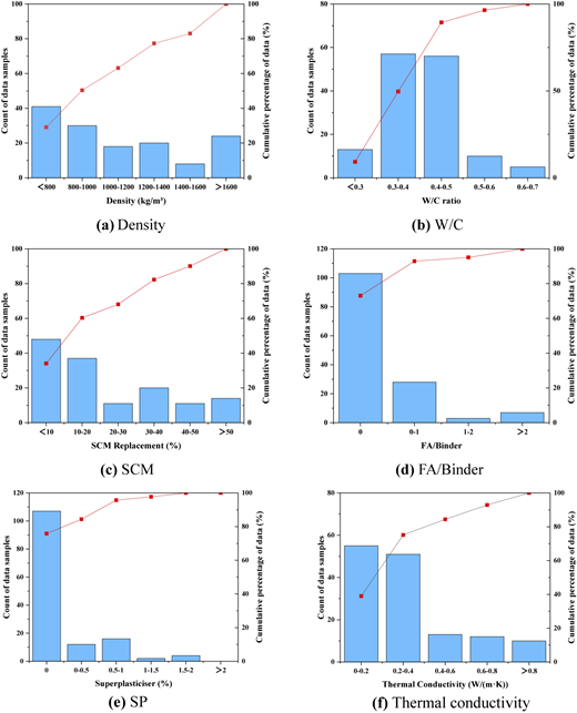
Figure 1 shows the distribution range of the thermal conductivity data. The density data were most densely distributed in the region below 800 kg/m³, with the number of samples decreasing as density increases (Figure 1a). Most of the W/C data were concentrated between 0.4 and 0.5, with fewer data at lower and higher ratios. The SCM replacement ratio data were concentrated in the low substitution region (<10%), with fewer samples at higher substitution rates, indicating that low substitution rate samples account for a larger proportion in the data (Figure 1c). The majority of data samples had an FA/Binder ratio of 0, suggesting that the FA content in this variable was relatively low (Figure 1d). SP content was mostly concentrated at 0%, with fewer data points in the other intervals (Figure 1e). Most of the thermal conductivity data were concentrated in the low thermal conductivity range (0–0.2 W/(m·K)), and as the thermal conductivity increased, the sample size gradually decreased, indicating that most studies focused on low-density, low-thermal-conductivity foam concrete (Figure 1f).

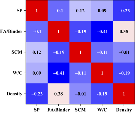
To avoid overfitting or computational instability in the model, this study conducted a correlation analysis on the parameters affecting the thermal conductivity (Figure 2) of foam concrete. It is clear that the correlations between the parameters were acceptable (i.e. <0.8), and thus the independence of each feature could be preserved during the machine learning modeling process, ensuring the accuracy of the prediction model.

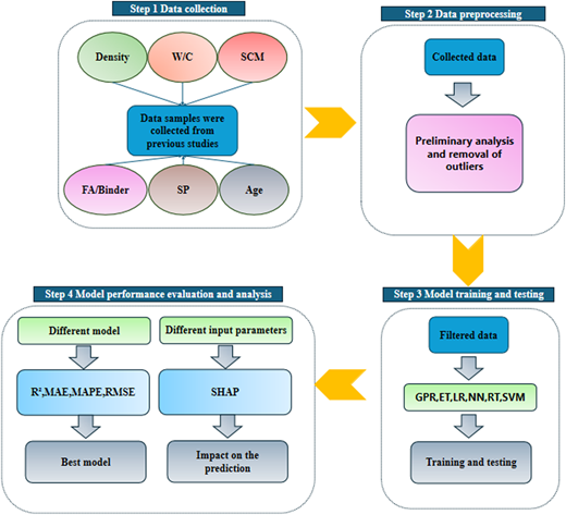
This study adopted a systematic approach to predict the thermal conductivity of foam concrete and evaluated the predictive models. As shown in Figure 3, the process was divided into four main parts: (1) data collection, (2) data preprocessing, (3) model training and testing, and (4) model performance evaluation and analysis.

A total of 141 datasets were systematically collected from previously published articles on the thermal properties of foam concrete (Maglad et al., 2023; Makul and Sua-iam, 2016; Ahmadi et al., 2023; Chung et al., 2019; Gökçe et al., 2019; Gencel et al., 2021; Vinith Kumar et al., 2018; Maglad et al., 2024; Jose et al., 2021; Özkan et al., 2024; Dora et al., 2025; Wei et al., 2024; Mydin et al., 2023; Azree Othuman Mydin et al., 2024; Bie et al., 2024; Xian et al., 2022; Shi et al., 2012; Changhui et al., 2024; Dianlong, 2017; Dingqiang et al., 2025; Ming et al., 2013; Tugen et al., 2024; Xiangming et al., 2019; Xing-xing et al., 2022; Yuejun et al., 2020). These data were carefully selected to ensure consistency in experimental conditions and methodologies, thereby ensuring the uniformity and reliability across different studies.

To reduce the impact of data heterogeneity from different sources on the results, several measures were implemented in this study. First, research data with clear experimental methods and consistent measurement standards were selected. Additionally, all numerical input data were standardized, and obvious outliers were excluded. These data processing steps ensured both the physical comparability and statistical consistency of the data, thereby enhancing the stability and generalization ability of the model training process.

To mitigate overfitting, this study used 5-fold cross-validation. The dataset was divided into five subsets, with one used for validation and the others for training in each experiment. This approach allowed evaluation on multiple data subsets, improving model generalization and reducing biases from specific data splits (Hu et al., 2025; Yu et al., 2025c). It also ensured stable and reliable model performance, providing more accurate assessment during training (Li et al., 2024; Sejuti and Islam, 2023).

GPR is a Bayesian non-parametric method (Shah et al., 2014) selected for its strength in handling uncertainty and fitting complex, noisy data often seen in concrete material studies (Ayyanar and Ali, 2024; Rayjada et al., 2023; Zhang, 2023; Wang et al., 2024b). Prediction is performed by modeling the training data with a Gaussian process. The core idea is to describe the correlation between data points through a covariance function. During prediction, not only the mean is provided but also the variance of the output. The core formula is as follows:

In this equation, $m(x)$ is the mean function, typically set to 0, and $k(x,x′)$ is the kernel function, which defines the correlation between data points. $K(X,X)$ represents the covariance matrix between the training data, while $σn2$ denotes the noise variance.

ET is a machine learning approach that combines multiple decision trees to improve prediction accuracy and stability. Using ensemble techniques like random forests or gradient boosting, each tree is trained on different data subsets, and the final prediction is derived from majority voting or weighted averaging. The core formula is as follows:

Assuming there are T trees, with each tree's prediction denoted as $ft(x)$⁠, the ensemble prediction is given by:

The trees in ET are generated through random sampling of the data. For classification tasks, the final output is the majority class voted on by all the trees:

where $I$ is the indicator function, representing whether the tree predicts the class $y$⁠.

LR is a statistical model used for predicting numerical outputs, assuming a linear relationship between the independent and dependent variables. The LR model finds the optimal model parameters by minimizing the loss function (usually the mean squared error), thereby making predictions. The core formula is as follows:

In this equation, $y$ represents the target variable, $x1$⁠, $x2$⁠, …, $xn$ are the feature variables, $β0$⁠, $β1$⁠, …, $βn$ are the regression coefficients, and $ϵ$ is the error term. $X$ is the matrix containing all the feature data from the training set, $y$ denotes the values of the target variable, and $βˆ$ represents the estimated regression coefficients of the model.

NN is a machine learning model that mimics biological neural networks, learning complex data patterns through multiple layers of nonlinear transformations. It consists of an input layer, hidden layers and an output layer, with neurons connected by weights and biases. The backpropagation algorithm optimizes the weights during training to minimize prediction errors. The core formula is as follows:

In this equation, $W$ represents the weight matrix, $x$ denotes the input, $b$ is the bias, $σ$ is the activation function, $L$ is the loss function and $η$ is the learning rate.

RT is a tree-based algorithm used for predicting continuous output variables. It recursively divides the data into different regions, where the predicted value for each region is the average of the data points within that region. The RT selects the best splitting features and thresholds by minimizing the squared error within each node. The core formula is as follows:

In this equation, $yˆ$ represents the predicted value, $N$ is the number of samples in the node and $yi$ denotes the true value of each sample.

SVM is a supervised learning method used for classification and regression analysis. SVM works by finding an optimal hyperplane that separates data points from different classes and maximizes the margin between them. For nonlinear separable problems, SVM utilizes a kernel function to map the data into a higher-dimensional space, where a linear hyperplane can then be found. The core formula is as follows:

In this equation, $ω$ represents the hyperplane vector, $b$ is the bias term, $ξ,ξ*$ are slack variables used to tolerate certain prediction errors and $C$ is the penalty factor, which balances margin maximization with error tolerance. $μAi(x)$ is the membership function of input $x$ to the fuzzy set $Ai$⁠, and $μBj(y)$ is the membership function of input $y$ to the fuzzy set $Bj$⁠. Their product represents the joint membership degree of $x$ belonging to $Ai$ and $y$ belonging to $Bj$⁠.

In order to evaluate the model accuracy, coefficient of determination (R²), root mean squared error (RMSE), mean absolute error (MAE) and mean absolute percentage error (MAPE) were used in this study. Table 2 summarizes the statistical evaluation metrics of different prediction models.

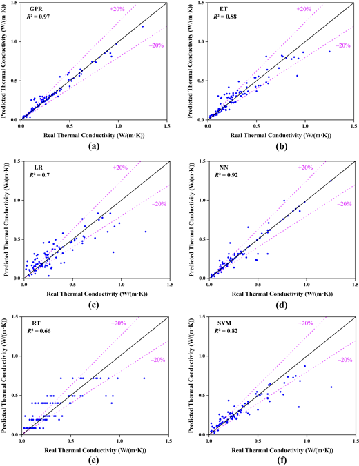
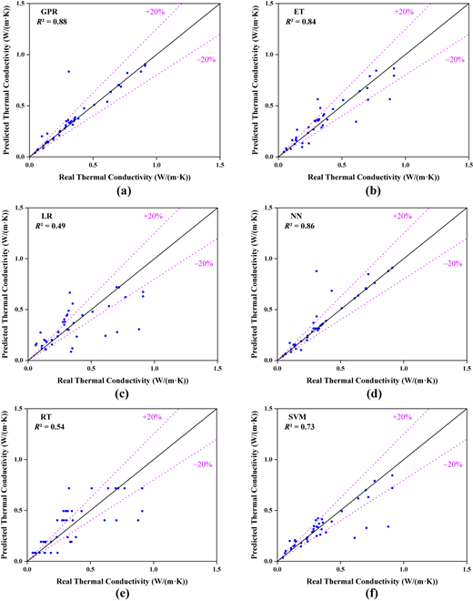
Figures 4 and 5 show the predicted vs. actual thermal conductivity values for six models in both training and testing phases. In the training phase, GPR and NN had the most concentrated points near the ideal line (y = x), indicating high fitting accuracy. SVM and ET also showed good fitting, while LR and RT displayed more scattered points, indicating poorer performance. In the testing phase, GPR and NN continued to perform well, with most points within the ±20% error range, showing strong generalization. ET and SVM had more dispersed points but were still close to the diagonal, while LR and RT had significant deviations, indicating unstable predictions and larger errors.

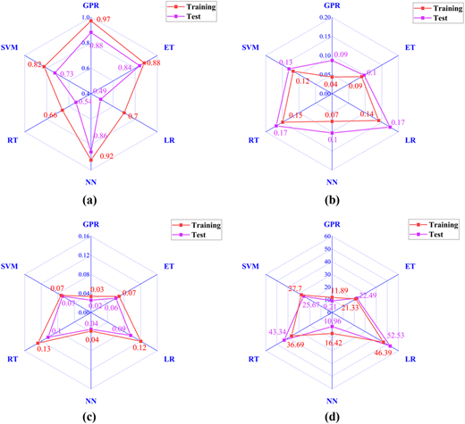
Figure 6 presents the specific R², RMSE, MAE and MAPE values for the six models (GPR, ET, LR, NN, RT and SVM) during both the training and testing phases when predicting the thermal conductivity of foam concrete. It is clear that GPR performed the best. Its R² value reached 0.9719 in the training phase and remained at 0.8814 in the testing phase, with RMSE and MAE values of 0.0437 and 0.0258, respectively, demonstrating its superior fitting ability, low error and good generalization capability. In comparison, ET and SVM also performed well in the testing phase; although their errors were slightly higher than GPR's, they maintained stability and were suitable for practical applications. However, LR and RT showed weaker performance in both the training and testing phases, particularly in the testing phase. LR had a MAPE as high as 52.53%, and RT's R² was only 0.5363, indicating significant overfitting issues for both models, poor prediction accuracy and weak generalization ability.

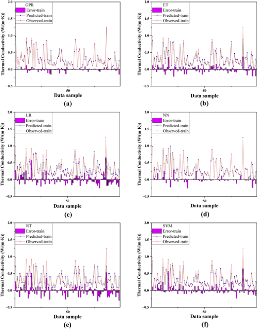
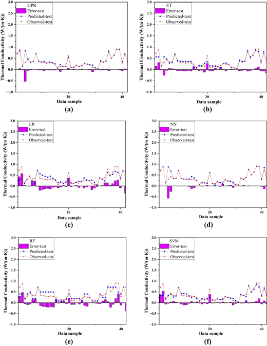
From Figures 7 and 8, the error plots reveal that GPR had low overall errors and stable predictions during both training and testing, indicating high accuracy, strong fitting and robust generalization. SVM's errors were moderate in training and slightly increased in testing, showing good generalization. NN had very low errors in training but significant error increases and fluctuations during testing, indicating overfitting. LR showed moderate training errors with larger fluctuations in testing, suggesting weak generalization. ET had higher errors in both phases, with considerable fluctuations in testing, indicating poor fitting and generalization. RT exhibited large errors and severe fluctuations in testing, reflecting weak performance and poor adaptability.

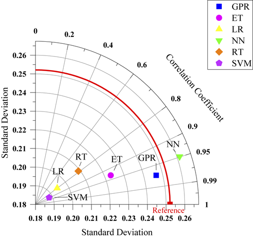
Figure 9 shows the Taylor diagram used for evaluating models’ predictive performance for thermal conductivity against reference values. GPR was closest to the reference, with a high correlation (close to 1) and a standard deviation consistent with the reference data, indicating its excellent accuracy and stability. NN, while also highly correlated, had a slightly higher standard deviation, making it less stable than GPR. ET and RT models deviated significantly, showing weaker predictive performance. LR and SVM had small standard deviations but risked underfitting. Overall, GPR provided the best balance of accuracy and stability.

Based on the comprehensive analysis above, GPR demonstrated the best fitting ability and generalization performance. Both SVM and NN also performed well; although NN showed some overfitting during the testing phase, the overall predictive performance remained satisfactory. The performance of ET was relatively average, with slightly higher errors, but there was no significant overfitting issue. LR and RT performed poorly in prediction, especially LR, which had weak generalization ability, and RT experienced severe overfitting, making them unsuitable for predicting thermal conductivity.

The results can be attributed to GPR, which, based on Bayesian optimization, accurately tunes key hyperparameters to better fit complex nonlinear relationships (Cheng et al., 2025). SVM performed well when parameters were adjusted, avoiding overfitting, but its generalization ability depends on the C value and kernel function. A larger C value can cause overfitting, while a smaller one may lead to underfitting. NN experienced overfitting, increasing testing errors. The LR model was too simplistic, failing to capture complex nonlinear relationships. ET and RT models, due to high randomness, performed poorly on some datasets. Therefore, GPR was the optimal model for predicting the flexural strength of foam concrete.

To further evaluate the robustness and generalization capability of the GPR model, different data-splitting ratios were adopted for model training and testing. In addition to the 60:40 division, the dataset was further divided into 70:30 and 80:20 ratios for comparison. The model performance under each partition was assessed using RMSE, R², MAE and MAPE. The corresponding results are summarized in Table 3.

As shown, the GPR model maintained stable prediction accuracy across all data division ratios, with R² values consistently above 0.90 and low RMSE and MAE values in both training and testing stages. These results indicate that the model exhibits strong robustness and reliable generalization performance, confirming its suitability for predicting the thermal conductivity of foam concrete.

SHAP is a model interpretation method based on game theory, which evaluates the contribution of features to prediction results by calculating their Shapley values. Positive contributions increase the predicted value, while negative contributions decrease it. SHAP provides transparent explanations for individual predictions (Rodríguez-Pérez and Bajorath, 2020) and assesses the global importance of features, thereby enhancing model interpretability and transparency (Flora et al., 2024; Scheda and Diciotti, 2022). Additionally, SHAP can reveal the interactions between features and potential biases, improving the reliability of the model. SHAP requires low correlation among input features (Indra et al., 2024). In this study, a correlation analysis was conducted prior to SHAP analysis, and the results indicated low correlation among input parameters, ensuring the accuracy of the analysis.

SHAP analysis was not limited to evaluating feature importance but was further employed to investigate the underlying physical mechanisms and the interactions among mix design parameters. Wang et al. (2023b) used SHAP to reveal both global and local effects of material variables on the compressive strength of recycled brick aggregate concrete. Following the same analytical approach, this study aims to elucidate how each variable affects the thermal conductivity of foam concrete.

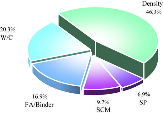
Figure 10 summarizes the global SHAP attributions for predicting the thermal conductivity of foam concrete. The percentage next to each variable indicates its relative contribution to the model output: density accounts for 46.3%, W/C for 20.3%, FA/Binder ratio for 16.9%, SCM replacement ratio for 9.7% and SP for 6.9%. These values quantify the average contribution of each parameter in shifting the model prediction from the baseline, thus reflecting its overall influence on model performance.

The density of foam concrete determines the volume fraction of air voids related to solid material. Thermal conductivity in foam concrete is primarily governed by porosity — a higher air content provides more insulation and reduces heat conduction paths, while denser materials contain more continuous solid phases that facilitate heat transfer. The W/C controls pore structure and hydration behavior. A higher W/C increases pore volume and connectivity and may reduce hydration density, thereby enhancing heat conduction through interconnected pores. Zhang et al. (2020) identified density and W/C as key factors influencing thermal conductivity. The FA/Binder ratio contributes 16.9%, reflecting the effect of the relative proportions of fine aggregate and binder. Since fine aggregate has a higher intrinsic thermal conductivity than the cement matrix, an increased FA/Binder ratio enhances solid-phase conduction and raises overall conductivity. The SCM replacement ratio contributes 9.7%, as SCMs primarily influence thermal behavior indirectly through pozzolanic reactions that alter hydration products and refine pore structures over time. Such effects are weaker in steady-state conductivity than those of density or W/C. SP shows the smallest contribution (6.9%) because it mainly improves the workability of fresh mixtures and has limited influence on the microstructure or thermal properties of the hardened concrete. Maglad et al. (2023) found similar limited effects of SCM on thermal conductivity, with Zhang et al. (2020) noting that SP had less influence than density or W/C.

In summary, SHAP provides a quantitative ranking of input parameters and links their statistical importance to the corresponding physical mechanisms. The dominance of density and W/C highlights their decisive roles in controlling the heat transfer performance of foam concrete, while SCM and SP exhibit secondary effects, consistent with previous experimental findings.

This study conducted a comparative analysis of the performance of different models in predicting the thermal conductivity of foam concrete under multiple input parameters. The optimal model for different output parameters was selected and subjected to sensitivity analysis. The conclusions are as follows.

1. Compared to most of the existing literature focusing on the prediction of compressive strength of foam concrete, this study shifted the objective to the prediction of the thermal conductivity. The input parameters selected include density, W/C, SCM replacement ratio, FA/Binder, SP and curing time. This approach significantly enhanced the dimensional richness of the model inputs and more effectively captured the nonlinear relationships between the multiple performance characteristics of foam concrete.

2. Through a comparison of six models—GPR, ET, LR, NN, RT and SVM—in predicting the thermal conductivity of foam concrete, this study found that the GPR model consistently outperformed the others in predicting thermal conductivity. The training phase produced R², RMSE, MAE, and MAPE values of 0.97, 0.04, 0.03 and 11.89, respectively, while the testing phase yielded values of 0.88, 0.09, 0.03 and 9.21. GPR demonstrated excellent fitting ability and robustness in handling high-dimensional nonlinear relationships, making it well-suited for the complex and noisy data characteristics associated with foam concrete's input parameters.

3. To enhance the interpretability of the model, this study employed the SHAP method to analyze feature contributions in the GPR model. The results indicate that the density and W/C were the primary factors influencing the thermal conductivity of foam concrete, while the SCM replacement ratio and SP had the least impact on the prediction outcomes. The contribution values of density and W/C were 46.3 and 20.3%, respectively, while the contributions of SCM replacement ratio and SP were 9.7 and 6.9%. This analysis provided a theoretical basis for the performance regulation of foam concrete in engineering practice.

In future research, additional experimental tests on the thermal conductivity of foamed concrete will be conducted to enrich the dataset and further validate the robustness and generalization capability of the models. By including a wider range of mix proportions and curing conditions, the variability in thermal behavior can be more comprehensively captured. Furthermore, inspired by recent advances in AI, we plan to introduce more advanced prediction models, such as ensemble learning, deep learning and hybrid intelligent systems, to further enhance prediction accuracy and methodological innovation. Comparative analyses with these advanced algorithms will also be conducted to evaluate their applicability to foamed concrete.

Although this study successfully developed and evaluated machine learning models for predicting the thermal conductivity of foam concrete, it primarily focused on a single thermal property. In future work, inspired by previous multi-objective studies (Wang et al., 2023a, 2024d), the dataset will be expanded to include mechanical and durability indicators such as compressive strength, density, water absorption and shrinkage. This will enable the establishment of multi-objective predictive models to jointly optimize thermal, mechanical and durability performance, providing a more comprehensive understanding of the structure–property relationships of foam concrete.