


This study seeks to foster fresh and exhaustive empirical relational evidence on the dynamism among oil price ripples, inflationary shocks and stock price volatility in India considering the time varying model along with vector autoregressive specification.
The study uses a time series econometrics technique covering the monthly data from January, 2006 to June, 2022. For the long-run results, vector error correction model (VECM) and for causal relationship, Granger causality test have been applied. Moreover, for robustness variance decomposition analysis (VDA) and impulse response function (IRF) are used by the authors.
Using Johansen’s co-integration test and VECM, the study documents that, there exists a unidirectional long-run causality from oil price and stock price to inflation. Additionally, the Granger causality test reveals a short-run bidirectional causal association between oil price and stock price; however, inflation does not influence any of the variables. Moreover, the VDA documents strong endogeneity of stock prices and strong exogeneity of inflation. Though, IRF almost validates the VECM results.
By seeing the interaction of stock prices with oil and inflation, investors and portfolio managers can forecast the movement of price and can accordingly take the decision.
The study concludes that a hike in the oil prices and a boom in the stock price jointly reinforce the inflationary situation over a longer time span in this country. Thus, the vitality of crude prices in controlling inflation and gauging the business cycle to ensure greater stability still remains a matter of high concern.
Introduction
Crude oil is the prime source of energy and indispensable input for production. Oil prices are considered as a primary macroeconomic factor indicating that they have the power to impact the global economic, financial stability and macroeconomic policies (Naifar and Al Dohaiman, 2013). Rising oil prices lead to higher cost of operation, changing corporate earnings (Maghyereh, 2006) which ultimately fuels the inflation (Hosseini et al., 2011; Aydoğan et al., 2017) and subsequently results in demand for higher wages to maintain the same standard of living which again fuels the inflation. This further leads to a lower demand for ultimate goods and services (Chittedi, 2012). Additionally, to curb the inflation government as per policy measures enhances the interest rate that drives the discounting rate used in the equity pricing formula (Kapusuzoglu, 2011; Sahu et al., 2015) and high-interest rates may discourage firms from investing, which ultimately affects the level of output. Another way, increasing oil prices also widen the current account deficits of oil-importing countries like India, which forces the government to devalue its currency (Shafi et al., 2015; Ghosh and Kanjilal, 2016; Sriram, 2015). Again, rising oil prices affect corporates via another mode, that is, due to higher oil prices firms buy less energy than before, hence overall productivity or collective supply of the firms decline (Cuñado and de Gracia, 2003; Sharma and Khanna, 2012). These above-mentioned phenomena pointedly impact the stock prices as they reflect the value of estimated future profits of the companies.
Besides it, the effect of rising oil prices on emerging oil-importing countries is more severe than that on developed countries as developing country’s demand are rising and they are more dependent on imported oil (Shafi et al., 2015). Moreover, Rahman (2020) disclosed that it is not possible for oil-importing countries to cut the demand despite rises in the prices of global crude oil. In emerging countries like India, higher demand for crude oil without the counterbalancing supply paves the way for inflation (Mitra, 2018). Ultimately, it is realized that the inflation rate and oil prices are interrelated to each other in a cause-and-effect relationship.
On the other hand, inflation is the result of a rise in price level, which in real sense lessens the purchasing power of the currency. Forecasting the inflation significantly increases speculation in the stock market among the traders. According to Sahu (2016), inflation is likely to impact the share prices either directly through the change in the price level or indirectly through the framework of policies outlined by the government to regulate it.
Generally, stock markets are termed as a leading sentiment of economic proposition, which focuses on the economic conditions of an economy. Fluctuations in the activities of equity segment change the confidence or sentiment of investors, which further shapes their spending pattern and affects corporate profitability (Audi et al., 2025). Explicitly, stock markets of any economy are affected by firm related variables, industry related variables and the macroeconomic variables (Anchal, 2017). Furthermore, Lee et al. (1995) have stated that, positive shocks in oil prices have a powerful influence than negative normalized shocks on growth. Through the variations in oil prices, stock indices of a country provide signal about the future path of an economy (Rahman, 2020). However, according to Kilian and Park (2009), the yields of the equity segment are dependent on the ultimate cause of oil price shocks. Sometimes, the movements in stock prices are taken as a significant aspect of understanding the variations in oil prices (Sahu et al., 2014). Though, depending on the economic circumstances of any country, the nature of linkage among macroeconomic variables and equity price varies. Therefore, the interrelationship among the international oil price fluctuation, inflationary situation and instability in the financial market of an economy has been a matter of debate for the past couple of decades concerning the demand–supply situation, pre–post liberalization periods, oil importing–exporting countries’ point-of-view and many other perspectives. As a major importer of crude oil, India has also witnessed this controversy among the development economists over the three decades after the convergence of the economy toward the global economy.
Furthermore, the recent Russia–Ukraine war and COVID-19 outbreak throughout the globe sharply hampered the global trade and hence growth. India is not outside the scenario of uncertainty and downward pressures generated through the geo-political tension. This crisis has created huge pressure in the oil market, stock market, demand and supply conditions and finally leads to the erosion of the standard of living even though the trend of inflation is downward. Overall, theoretical propositions are now in question. Despite their enormous individual importance, such as oil serving as economic life-blood, inflation acting as the economy’s body temperature and the stock market functioning as a barometer of the economy, the investigation of the linkages, interactions and combined impact on each other has gained a greater role in enhancing the overall economic well-being. In this purview, this study seeks to foster fresh and exhaustive empirical relational evidence on the dynamism among oil price ripples, inflationary shocks and stock price volatility in India considering the time varying model along with “Vector Autoregressive” (VAR) specification covering the maximum possible monthly data series.
Literature review
Over the last couple of decades, there has been a rising number of published research papers in the prevailing literature covering the nexus between oil price variations and share prices. But, with the changing environment, the relationship of share prices with various other macroeconomic variables has been a most important area of hypothetical and empirical investigation. Empirical investigation of the dynamic associations among macro-economic indicators and equity prices has grown considerably with the supposition that variation in securities prices is an imperative gauge of economic activity. Therefore, a wide range of prior research studies have been drawn here in the context of various counties economy apart from India and in different time frames.
The bearing of several macroeconomic indicators on the securities prices has been considered by Singh (2010). The study reveals that the only variable with feedback causality with Sensex is the IIP. Further on, the study of Tripathy (2011) found that, equity market, Bombay stock exchange (BSE) volume and interest rate cause each other. Additionally, the study discloses that the Indian stock market is not efficient in weak form. Liu et al. (2023) have observed the increased sensitiveness of the stock market to the oil price variations during the times of economic policy uncertainty. Additionally, the response of securities market is asymmetric in various industries in China. By taking oil price, domestic gold price and stock indices, Bhunia (2013) observes the long-term association among the variables in the scope of India. Considering data over the period from January 2000 to November 2018, Aggarwal and Manish (2020) have finally come to an end with the insignificant influence of exchange rate and adverse influence of inflation and real interest rate on the share index. Further, this study also documents a positive association between the BSE index and oil price.
Another remarkable study has been passed on by Hosseini et al. (2011) in the context of two developing countries economy namely, India and China. This empirical study found that there is a connection between the four undertaken macroeconomic indicators and equity market indicators in both economies. Further, the study resolved that, the impact of inflation, money supply and crude oil price is augmenting and the effect of IIP is harmful in China. But in the Indian context, these impacts are quite different. The influence of IIP and the inflation is positive, whereas the impact of money supply and oil is negative. The study of Castro and Jiménez-Rodríguez (2024) have highlighted the impact of oil price shocks (demand shocks and supply shocks) underlining the role of oil inventories. The study concluded that stock returns remain unaltered by the types of oil price shocks given the explicit consideration of oil inventories in the model. Similarly, a depth study with respect to various oil price shocks (supply, demand and risk shock) on the stock market of China was explored by Ge (2023). Outcome revealed that oil price shocks have heterogeneous impact on the different states of the market, i.e. bullish and bearish.
Apart from India, we are now discussing other studies that are in the literature focusing on the relationship among macroeconomic indicators and securities prices. Starting from China, which is one of the developing nations of Asia, Du et al. (2010) have examined that the world oil price drives the growth rate of economy and inflation rate, even though the impact is non-linear. But on the other side, the economy of china does not affect the international oil price. Likewise, Kwon and Shin (1999) have observed that the macroeconomic indicators reflect the Korean equity market. Taking into consideration the multivariate vector-autoregression approach, Papapetrou (2001) tries to look into the relationship and ultimately concluded that oil prices play a substantial role in the economic activity and employment of Greece. Abuoliem et al. (2019) have documented in the context of Jordan, the association among global and domestic macroeconomic parameters and financial sector index. Finally, this study concluded that the global oil price and producer price index have a detrimental effect and inflation rate has a statistically non-significant influence on the financial index.
Through the detailed survey of previous literature, the study of Degiannakis et al. (2018) has documented that, the varying association between oil price and stock index is mainly due to the types of stock indices considered (i.e. aggregate or sectoral), types of country (oil-importing or oil-exporting) and nature of changes in oil prices. Berument and Taşçı (2002) have targeted to explain the consequence of oil prices on the general price level in their study. At the end, they suggested that, the extent to which crude oil prices move the general price may be subject to the wage rate and other income-associated factors held responsible for the general price level for Turkey. Likewise, Ali (2011) has found that inflation and foreign remittance have an adverse impact on the stock returns of the Dhaka Stock Exchange. Furthermore, Sadorsky (2003) examined the responses to the shocks of three key macroeconomic variables, i.e. oil price, the term premium and the inflation on the Pacific stock exchange index. The statistical outcomes indicate that each and every variable has a noteworthy effect on the volatility of Pacific stock exchange technology stock prices.
Asprem (1989), by considering ten European countries, has demonstrated that import level, inflation rate, employment and interest rate are adversely connected with the share prices. Ultimately, it is evident from the portfolio of European stock indices that this portfolio strongly explains the variation in stock prices. In line with the previous study done by Asprem (1989), Cuñado and de Gracia (2003) have also attempted to inspect the influence of oil prices on the inflation rate and IIP for several European countries and finally show that oil prices have a substantial bearing on the inflation and non-symmetric effect on the growth rate of production. Employing the GSADF model, Khan et al. (2021) have detected the existence of numerous oil price bubbles. The start and end of a particular bubble are associated with a specific crisis. Besides, the other factors that contribute toward the bubbles are interruption of oil demand and supply, dollar depreciation and expansion of the global economy.
Considering the EGARCH model, the study of Erdem et al. (2005) at the end documented the presence of unidirectional volatility spillover from the inflation rate to stock market indices. On the framework of the Norwegian stock market, Gjerde and Saettem (1999) have demonstrated that, real interest rate change influences both equity market yields and the rate of inflation and that the equity market also responds to the variations in oil prices. According to Humpe and Macmillan (2009), securities prices are positively interrelated with the industrial production of both countries, i.e. the USA and Japan. Furthermore, stock prices are adversely interrelated with the inflation and rate of long-term interest in the USA, but in Japan, industrial production is adversely connected with the long-term rate of interest and inflation. The influence of crude oil price and bitcoin on the equity return volatility has been measured by Mishra and Dash (2024). The study presented the existence of volatility spillover over a long period of time from crude oil to the selected eight Asian stock exchanges and from bitcoin to all stock exchanges except Malaysia.
In the context of Russia, Ito (2012) found that in a short period of time, inflation was negatively and economic growth was positively related to the oil prices. In the Iranian economy, Farzanegan and Markwardt (2009) revealed that oil price variations remarkably increase inflation and after that terminate with the positive linkage between oil price oscillations and industrial output. In the context of a developing oil-exporter country that is Nigeria, Iwayemi and Fowowe (2011) conducted an empirical study and concluded that most of the macroeconomic indicators, such as output growth, public expenditure, inflation rate and the real rate of exchange, are not meaningfully impacted by the positive shocks in oil prices. However, oil price variations act as obstacles for the output and rate of real exchange. In the same way, Heinlein and Mahadeo (2025) have checked the association of crude oil and US stock return in the regimes of low and high oil price uncertainty by considering the VAR model.
Through a rigorous review of literature varying with respect to country’s socio-economic condition, macroeconomic environment, specification of time and application of methodology, we observe heterogeneous and inconclusive findings from a global perspective including India. Besides, to decide upon the overall impact of all the variables on the Indian economy, such as linkage, interaction, reflection or absorbing tendency tracing through a dynamic framework is not properly stated. Moreover, studies on the joint impact of crude oil price and inflation, which are the fundamental macroeconomic variables, on securities prices, especially for developing countries like India, are still lacking. Hence, it is imperative in today’s globalized era for equity players and policymakers to recognize the macroeconomic parameters on the movements of share prices for managing their financial decisions. In this background, the study is an attempt to explore the relationships among crude oil prices, inflation and share prices and bridging the gap that existed in the literature.
Data and methodology
To investigate the trilobite dynamic relationship among crude price ripples, stock price volatility and inflation shocks in the Indian contest, the study considers maximum possible data in the monthly frequency over the period from January 2006 to June 2022. Considering the economic relevance as well as the degree of impact on the Indian economy, the study proxies NIFTY-FIFTY as an indicator of stock price movement and represents the CPI (“Consumer Price Index”) as an indicator of Inflation undulation. Besides, the study considers the Brent oil price per barrel as an indicator of international oil prices. The NIFTY, CPI and Brent crude prices have been compiled from NSE, RBI and World Bank databases, respectively.
The empirical approach employed in this research basically follows the previous work of Agarwalla et al. (2021). Therefore, given the relationship and dynamism among the variables over the time, it is also relevant to apply VAR comprehensively. Since, the VAR is reasonably recognized and thoroughly documented in our previous work, only a concise overview is presented.
The study at first estimates the “Descriptive Statistics” to observe the prime characteristics of the modeled variables and examine “Unit Root Test” to know order of integration or stationary properties. This would help us in finding the order of integration and hence employ the co-integration test. After that, based on the result, “vector error correction model” (VECM), “variance decomposition test” (VDT) and “impulse response function” (IRF) were employed to frame the long and short-run dynamism among crude prices, inflation and stock prices and to detect the direction of the relationship.
Stationarity or the order of integration is the prerequisite under the VAR model to draw justifiable inferences and to augment the accuracy and consistency of the model constructed. However, “Augmented Dickey-Fuller” (ADF) test and “Phillips-Perron” (PP) test have been considered to identify the stationarity property.
The use of lag length in the VAR model is both sensitive and decisive criterion. Therefore, prior to estimation, it is inevitable to determine the appropriate lag length. Having identified the proper lag, VAR based co-integration test (Johansen, 1988), has been applied to examine the dynamic relationship among crude price, inflation and stock price movements. This approach is built on the following autoregressive mechanism:
Where Yt represents the vector having n number of first order integrated variables and subscript t is the time period. μ is a vector of (n × 1) constants, Ap represents (n × n) matrix of coefficients, with respect to the maximum lag p. The above VAR can be replaced by the following error correction framework:
Where, details the short-run dynamics and signifies the long-run kinetics within the set of variables embodied in the vector Yt and I indicate identity vector. Besides, this process traces out the independent co-integrating vectors through the rank of matrix, .
The nature of the long-run relationship may differ with the short-run dynamics. Therefore, this study adopts “Vector Error Correction” (VEC) mechanism to explore the short-run dynamics among oil prices, inflation and share indices. The VEC mechanism is based on restricted VAR, which best deals with co-integrated non-stationary series. The error correction term (ECT) observed through the VEC mechanism describes the rate of adjustment at which it pulls back to its long-run equilibrium.
Thereafter, the study estimates diagnostic tests to validate the VECM.
Further, this analysis needs to uncover the strength of the exogeneity of the variables beyond the sample period as well as the degree and direction of causality among crude price, inflation and share price. Therefore, this study employs VDT analysis to address the degree of exogeneity of the variables and identifies the relative importance of one variable in generating variances on other variables included in the system. Besides, the IRF depicts an improved understanding of both short- and long-run future impacts of innovations generated through the VAR system. The stability of the impression advocates how instantly the process returns to equilibrium.
Analysis and findings
The analysis begins with the descriptive statistics reported in Table 1. From the table, it is evident that all the concerned macro-economic variables, i.e. oil price, NIFTY and CPI, are not stable at all within the period under investigation. All the variables exhibit notably different values from their averages. First of all, the summary statistics of NIFTY, maximum index of 17671.65 and minimum index of 2755.10 with an average of 7879.585 points, explain its instability throughout the study period, which is further confirmed by the large standard deviation value (3739.393).
Summary statistics
| Statistics | NIFTY | Oil price | CPI |
|---|---|---|---|
| Mean | 7879.585 | 76.33359 | 236.7727 |
| Median | 6700.300 | 71.47500 | 242.5000 |
| Maximum | 17671.65 | 133.8700 | 373.0000 |
| Minimum | 2755.100 | 23.34000 | 119.0000 |
| Standard deviation | 3739.393 | 25.43749 | 74.78059 |
| Skewness | 0.896216 | 0.311642 | 0.008664 |
| Kurtosis | 3.120304 | 2.021598 | 1.795943 |
| Jarque–Bera test statistic | 26.62511 | 11.10247 | 11.96295 |
| Probability | 0.000002 | 0.003883 | 0.002525 |
| Observations | 198 | 198 | 198 |
Likewise, the instability of CPI and oil prices is also well documented, given the mean and standard deviation values ($236.77 and 76.33 pts) and ($ 74.78 and 25.46 pts), respectively.
Findings of long-run analysis
According to the stated objective, the study analyses exhaustive trilobate associations among the concerned macroeconomic variables.
The long-run investigation was performed through Johansen’s co-integration test after meeting the necessary preconditions. The test involves three main steps. Firstly, it determines the integrating order by employing the two different types of unit root test. Secondly, it estimates the suitable lag length, which confirms that projected residuals are free from autocorrelation. Lastly, we construct the co-integrating vectors under the VAR framework.
The reports of ADF and PP tests are depicted in Tables 2 and 3 exhibit that for all variables the null hypothesis in its levels cannot be rejected but at their first difference it is rejected for both the models at 5% significance level in both tests. Therefore, oil price, NIFTY and CPI are non-stationary to level and stationary in their first differences.
ADF test results
| Variables | Level | First difference | Result | ||
|---|---|---|---|---|---|
| I | IT | I | IT | ||
| NIFTY | −0.878433 (0.7939) | −3.062932 (0.1177) | −12.21566 (0.0000) | −12.16338 (0.0000) | I(1) |
| Oil price | −2.184989 (0.2124) | −1.912716 (0.6448) | −9.811534 (0.0000) | −9.859674 (0.0000) | I(1) |
| CPI | 3.551474 (1.0000) | −2.309360 (0.4268) | −2.597763 (0.0549) | −8.574196 (0.0000) | I(1) |
Note(s): (a) MacKinnon (1996) one-sided p-values; I(1) = Stationary at order one; I = Intercept and IT = Intercept and Trend
PP test results
| Variables | Level | First difference | Result | ||
|---|---|---|---|---|---|
| I | IT | I | IT | ||
| NIFTY | −0.902657 (0.7863) | −3.246798 (0.0779) | −12.21566 (0.0000) | −12.16338 (0.0000) | I(1) |
| Oil price | −2.010055 (0.2825) | −1.703892 (0.7468) | −9.567524 (0.0000) | −9.599316 (0.0000) | I(1) |
| CPI | 2.591976 (1.0000) | −1.947359 (0.6264) | −11.76449 (0.0000) | −12.03427 (0.0000) | I(1) |
Note(s): (b) MacKinnon (1996) one-sided p-values; I(1) = Stationary at order one; I = Intercept and IT = Intercept and Trend
Given its sensitivity to the selection of a best fit lag length, the study needs to determine the proper lag length before carrying out Johansen co-integration test. The outcomes of the AIC criteria are reflected in Table 4.
Lag order selection criteria for VAR
| Lag length | AIC |
|---|---|
| 0 | 37.40494 |
| 1 | 24.59397 |
| 2 | 24.41923 |
| 3 | 24.48220 |
| 4 | 24.53173 |
| 5 | 24.51877 |
| 6 | 24.50900 |
| 7 | 24.50189 |
| 8 | 24.39231* |
| 9 | 24.42613 |
| 10 | 24.43376 |
| 11 | 24.43126 |
| 12 | 24.42866 |
Showslag order indicated by the criterion
Considering all the statistics of the AIC criteria, the study prescribes eight as the optimum lag (at 5% level), as theory proposes smaller the statistics (24.39231) better fit the model.
After satisfying the stationary property and identifying the optimum lag, the study proceeds to implement the co-integration test to estimate the long-run common stochastic trend or co-movement among oil price, NIFTY and CPI.
The results described in the aforementioned Tables 5 and 6 indicate that the null hypothesis of this co-integration test of no co-integration among the variables undertaken is rejected at 5% significance level. Here, the critical values (29.79707 and 21.13162 respectively) of Mackinnon–Huag–Michelis are smaller than the computed values of Trace statistics [34.74190] and Maximum Eign statistics [26.83937] respectively. The co-integration results also confirm the existence of only one co-integrating vector, which indicates a long-run co-integrating relationship among the oil price, NIFTY and CPI. Finally, the co-integrating equation is formulated as follows:
“Johansen cointegration test” (trace statistics) result
| H0 | H1 | Trace statistics | 5% critical value | Prob. value* |
|---|---|---|---|---|
| r = 0 | r = 1 | 34.74190 | 29.79707 | 0.0124 |
| r ≤ 1 | r = 2 | 7.902533 | 15.49471 | 0.4759 |
Note(s): *p-values by MacKinnon-Haug-Michelis (1999)
“Johansen cointegration test” (maximum Eigen statistics) result
| H0 | H1 | Maximum Eigen statistics | 5% critical value | Prob. value* |
|---|---|---|---|---|
| r = 0 | r = 1 | 26.83937 | 21.13162 | 0.0070 |
| r ≤ 1 | r = 2 | 7.623098 | 14.26460 | 0.4183 |
Note(s): *p-values by MacKinnon-Haug-Michelis (1999)
The above co-integrating equation again confirms the significant and positive existence of long-run relationships having significant t-values at 5% level. So, in the long-run, variables collectively move in one direction.
Findings of short-run analysis
Having co-integration among the modeled variables, the study further moves ahead to document the trilobate short-run dynamism among oil price, NIFTY and CPI under the VEC mechanism.
Table 7 presents the t-values corresponding to the coefficients of the lag values of all the modeled variables under the VEC framework. This evidences that only the first lag value of oil price and forth lag value of NIFTY are statistically significant with negative signs when NIFTY and oil prices are considered as independent variables, respectively. Therefore, the short-run dynamics indicate that both oil price and NIFTY have significant and negative impacts on each other. Whereas, CPI does not have significant role, neither impacting nor being impacted by the other variables in the system.
Result of “vector error correction model”
| Independent variables | Dependent variables | ||
|---|---|---|---|
| D(NIFTY) | D(Oil price) | D(CPI) | |
| ECT () | −4.05E‐05 [−0.60935] | 1.57E‐06 [1.56402] | −1.41E‐06** [−5.46209] |
| D(NIFTY (−1)) | 0.085321 [1.07712] | −0.003951** [−3.29439] | 0.000224 [0.72806] |
| D(NIFTY (−2)) | −0.149724 [−1.84181] | −0.001336 [−1.08522] | −6.72E−05 [−0.21267] |
| D(NIFTY (−3)) | 0.073722 [0.89483] | 0.000522 [0.41841] | −2.77E−05 [−0.08643] |
| D(NIFTY (−4)) | −0.035177 [−0.43664] | 0.000277 [0.22678] | −0.000555 [−1.77186] |
| D(NIFTY (−5)) | −0.013752 [−0.17068] | 0.000924 [0.75727] | −0.000485 [−1.54750] |
| D(NIFTY (−6)) | −0.043407 [−0.53829] | 0.001961 [1.60590] | 0.000582 [1.85533] |
| D(NIFTY (−7)) | 0.112044 [1.36433] | 0.001618 [1.30118] | −4.10E−05 [−0.12829] |
| D(Oil price (−1)) | 7.002599 [1.51866] | 0.372757** [5.33957] | −0.003389 [−0.18908] |
| D(Oil price (−2)) | −2.776281 [−0.57036] | 0.015179 [0.20597] | 0.003774 [0.19943] |
| D(Oil price (−3)) | 3.560597 [0.73522] | −0.069888 [−0.95318] | 0.010136 [0.53835] |
| D(Oil price (−4)) | −12.78298* [−2.64297] | −0.054685 [−0.74681] | −0.009627 [−0.51203] |
| D(Oil price (−5)) | 5.313831 [1.08404] | 0.061001 [0.82196] | −0.016187 [−0.84946] |
| D(Oil price (−6)) | −8.478020 [−1.71428] | −0.148245 [−1.97991] | 0.007309 [0.38018] |
| D(Oil price (−7)) | −0.245776 [−0.05385] | 0.041780 [0.60461] | −0.017829 [−1.00484] |
| D(CPI (−1)) | 5.889045 [0.35437] | −0.002447 [−0.00973] | 0.252379** [3.90652] |
| D(CPI (−2)) | 4.413074 [0.26573] | 0.120188 [0.47801] | −0.097657 [−1.51261] |
| D(CPI (−3)) | −21.48608 [−1.35477] | 0.023979 [0.09987] | 0.005722 [0.09280] |
| D(CPI (−4)) | 0.953160 [0.06048] | −0.336404 [−1.40989] | −0.107521 [−1.75497] |
| D(CPI (−5)) | −12.62917 [−0.79265] | −0.295597 [−1.22542] | −0.271895** [−4.38971] |
| D(CPI (−6)) | 0.049809 [0.00302] | 0.223813 [0.89556] | 0.207363** [3.23142] |
| D(CPI (−7)) | −29.14921 [−1.77583] | 0.083338 [0.33535] | −0.385237** [−6.03714] |
| C | 81.65464 [1.78058] | −0.149552 [−0.21540] | 1.366357** [7.66432] |
Note(s): *** Statistically significant at 1% level; ** at 5% level; [ ] t-values
The t-values of ECT of the VEC mechanism show that CPI corrects the disturbances significantly to converge toward a long-run equilibrium situation and in the right path, but the oil price and NIFTY do not respond meaningfully. The approximate value of the coefficients of ECT of CPI is −1.41, which advocates the speed of adjustment per period, i.e. if any disequilibrium occurs in the short-period the model is pulled back to the equilibrium almost at 141% rate.
Diagnostic tests results
Table 8 reports the diagnostics estimates of VECM residuals, which confirm the proper specification of the model as well as the robustness of the VECM estimates considering results of “serial correlation test”, “normality test” and “heteroscedasticity test” estimated through “Lagrange-Multiplier Test” of residuals, “Jarque–Bera test” and “white heteroscedasticity test”, respectively. For all cases, the test statistics fail to reject the the assumptions of null hypothesis of “no serial correlation”, “normal” and “heteroskedasticity,” respectively.
Results of diagnostic tests
| VEC residual of | Serial correlation (1) | Normality (2) | Heteroscedasticity (3) |
|---|---|---|---|
| Oil price – NIFTY – CPI | 0.620042 (0.5458) | 14.125806 (0.1298) | 1.740456 (0.2012) |
Note(s): (1) “Lagrange Multiplier Test” of Residual “Serial Correlation”
(2) “Jarque–Bera Test” of Normality
(3) “White Heteroscedasticity Test” with no Cross Terms Yields
Respective values of Probability are shown in Parentheses
Furthermore, the VECM coefficients were tested through stability analysis by applying the CUSUM (“Cumulative Sum of Recursive Residuals”) test. The plot in Figure 1 confirms the stability of the parameters undertaken within the model over the study period.
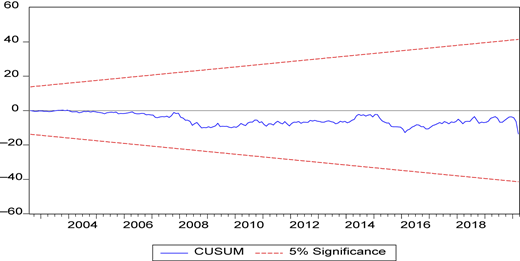
Plot of cumulative sum of recursive residuals for oil price, NIFTY and CPI. Source: Prepared by authors
Plot of cumulative sum of recursive residuals for oil price, NIFTY and CPI. Source: Prepared by authors
Findings from causality test
Since the model observes a co-integrating relationship among the modeled variables and conducts the VEC mechanism, the study applies Engle and Granger (1987) test instead of introducing a standard Granger test to avoid the misspecification problem in identifying the causal relationship among these macroeconomic variables.
Long-run causality
The presence of a significant unidirectional long-run causality from oil price and NIFTY to CPI is established through the t-value observed from ECM, which is reported in Table 7. The coefficient of the ECT -1.41 is significant at 1% level, which advocates that lubricity in oil prices and shocks in NIFTY indices instigate the inflationary situation in the long-run.
Short-run causality
The results of “VEC Granger Causality Test” are reported in Table 9, which exhibit a bidirectional causal relationship between NIFTY and oil price, i.e. both are influenced by each other and surprisingly, CPI is considered to be insignificant.
VEC “Granger causality test” result
| Dependent variables | Independent variables | Chi-square value | Prob. value | Outcome |
|---|---|---|---|---|
| NIFTY | D(Oil price) | 13.80647 | 0.0547 | Existence of causality |
| D(CPI) | 5.831404 | 0.5596 | No causality | |
| Oil Price | D(NIFTY) | 16.78126 | 0.0189 | Existence of causality |
| D(CPI) | 5.081864 | 0.6500 | No causality | |
| CPI | D(NIFTY) | 10.53568 | 0.1602 | No causality |
| D(Oil price) | 2.651162 | 0.9153 | No causality |
Reports of VDT and IRF
Having established the causal relationship, the investigation extends toward VDT and IRF analysis to estimate the degree of exogeneity and pulse of the relationship among oil price, NIFTY and CPI beyond the sample period.
Table 10 demonstrates that NIFTY exhibits strong endogeneity as nearly 96% of its deviation is accounted for by its own variance even after a two-year period, and in this same way, innovation in the Indian stock price itself is established as the main driver behind its volatility. Meanwhile, the explanatory power of oil price and CPI are found to be insignificant. Further, the decomposition result exhibits that a significant portion (almost 28%) of oil price is explained by NIFTY. The evidence also shows that within the time span CPI gradually lose (98 to 54%) its explanatory power, whereas oil price and NIFTY accounted for around 34 and 14% forecast error variances. However, this portion concludes that CPI is strongly exogenous and NIFTY behaves as strongly endogenous, i.e. NIFTY demonstrates greater self-dependent than its dependence on oil price and CPI.
Variance decomposition
| Variables | Period | % of estimate error variance | ||
|---|---|---|---|---|
| NIFTY | Oil price | CPI | ||
| NIFTY | 1 | 100.0000 | 0.000000 | 0.000000 |
| 4 | 98.55393 | 1.363765 | 0.082305 | |
| 8 | 97.48120 | 1.294925 | 1.223876 | |
| 12 | 96.07381 | 1.758205 | 2.167984 | |
| 16 | 96.42112 | 1.680381 | 1.898497 | |
| 20 | 96.38659 | 1.642278 | 1.971127 | |
| 24 | 96.37562 | 1.606290 | 2.018095 | |
| Oil price | 1 | 2.686079 | 97.31392 | 0.000000 |
| 4 | 10.71911 | 89.22086 | 0.060022 | |
| 8 | 15.59442 | 83.71712 | 0.688462 | |
| 12 | 23.11932 | 76.04150 | 0.839177 | |
| 16 | 25.57241 | 73.54480 | 0.882786 | |
| 20 | 26.92756 | 71.99912 | 1.073320 | |
| 24 | 27.81273 | 71.06965 | 1.117629 | |
| CPI | 1 | 2.366840 | 0.000359 | 97.63280 |
| 4 | 4.604269 | 1.914895 | 93.48084 | |
| 8 | 3.650203 | 7.805385 | 88.54441 | |
| 12 | 5.664727 | 13.45225 | 80.88302 | |
| 16 | 8.838775 | 20.09317 | 71.06805 | |
| 20 | 11.02034 | 26.71981 | 62.25985 | |
| 24 | 13.76157 | 32.31936 | 53.91907 | |
In Figure 2, the outcomes of the IRF analysis draft the lineal response of 24 months to a one standard deviation innovation alternatively in all the variables under the system. The responses engendered from a positive shock to CPI are almost the same for both the NIFTY and oil price, i.e. the response is positive only for the first few periods and then persistently negative almost at a constant level in the future periods. Although, a one standard deviation positive innovation in NIFTY generates an upward trend response for both oil price and CPI. Besides, almost a positive and inclining response in the CPI is observed when a shock is put to the oil price throughout the time horizon. Finally, this part of the analysis again justifies the VECM and variance decomposition results.
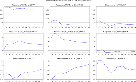
Impulse response function. Source: Prepared by authors
Impulse response function. Source: Prepared by authors
Conclusion and recommendations
The association between crude oil price and inflation and their relevance to forecast stock prices, is complex, comprehensive, multifaceted and dynamic. Our exploration into this topic has revealed that in the long-run the study documents a positive co-movement among oil price, inflation and equity price in India. However, as opposed to this findings, the study of Agarwalla et al. (2021) documented that the BSE energy index goes down by the upsurges in crude oil prices. This may so happen owing to the fact that, elevated oil prices are propelled by the worldwide boom period in which demand enhances significantly and it also fans the inflation with stock prices. Another way, inflation is positively related to the share prices, as if inflation is the result of increased money available in the economy or the initial upward phase of the growth of the economy, then inflation does not impact the consumer expenditure. Thereby, the sales revenue of the corporations increases, which is reflected in share prices. In addition, the VECM directs a long-run causal relation from oil price and stock price to inflation. As a crucial input in the process of production, oil price affects the cost of production and earning levels of the firm; hence, the share price and inflation level become affected. This finding is also consistent with Singh (2010), Tripathy (2011), who also revealed that the stock market has unidirectional causality with inflation.
However, considering the short-run dynamics, the results of VECM approve that both, oil price and NIFTY, have a statistically significant and negative impact on each other. Whereas, CPI does not have significant role, neither impacting nor being impacted by the other variables in the system. This result is quite deviated from the earlier results of long-run, as in short-run most of the companies fitting to various sectors of the economy are not able to change the selling rate in response with the fluctuations in the oil price; therefore, the retail price level, i.e. consumer price index, remains unchanged but the profit margin of the companies and thereafter stock prices fall down. Additionally, the causality test by Granger reports a short-run two-way causal association between the crude oil price and stock price, whereas inflation is not impacting any of the variables. Likewise, in a study, Tripathi and Seth (2014) have found that oil price has a both way causal association with the BSE Sensex. However, in contrast to this, Saxena and Bhadauriya (2012) have found that inflation and oil prices cause each other, which may be due to the changed time period under study. Additionally, the variance decomposition analysis (“VDA”) documents the strong endogeneity of share prices and exogeneity of inflation. Again, the analysis of IRF depicts that the responses engendered from a positive innovation of stock price to oil price and inflation are moderately positive while, the inclining response of inflation is observed for a shock to the oil price. Somehow at odds, a positive impulse to inflation generates a persistently negative response at a constant level in the Indian context. Therefore, in the end, for consumers, investors and policymakers, the crude oil price strikes its footstep. Thus, the vitality of crude prices to control over the inflation and to gauge the business cycle for ensuring greater stability still remains a matter of high concern for the policymakers and investors. Therefore, investors, policymakers and investment advisors in this respect are informed to take the investment decisions sensibly after considering these above-mentioned factors and their relationships.
This study is limited to India only, and combining it with other developing countries would enhance the scope for generalization of the results. Besides, the incorporation of other variables such as exchange rate, gold price, money supply, FDI inflows, etc. will provide a more robust result.

