


Based on unique panel data from a five-wave internet survey in Japan, we show how the coronavirus disease 2019 (COVID-19) pandemic affects people’s prospect-theory risk preferences, especially in the loss domain. The panel analysis indicates that following the spread of the pandemic, diminishing sensitivity becomes stronger for the participants’ value and probability weighting functions. Therefore, owing to the pandemic, (i) people become less sensitive to an increase in losses and feel less displeasure owing to losses, especially large ones, and (ii) they become more pessimistic toward losses occurring with tiny probabilities, and more optimistic toward losses with larger probabilities. One implication of the study is that people become less cautious about the risks of suffering large losses with non-tiny probabilities, which may slow down the recovery of society.
1 Introduction
It is critical to know the effects of pandemics and other external negative shocks on people’s risk attitudes. This is because personal risk preferences determine one’s preventive and precautionary behaviors against further spreading and the reoccurrence of shocks. This study aims (i) to show how the coronavirus disease 2019 (COVID-19, hereafter) affected people’s risk attitudes especially in the loss domain, and (ii) to ascertain the underlying shift in risk preferences, using the framework of prospect theory (Kahneman and Tversky, 1978; Tversky and Kahneman, 1992).1 We use unique panel data from a five-wave internet survey (N = 14, 470 for the balanced panel), conducted from March 2020, when the number of infected individuals began increasing sharply, to June 2020, when the infection rate remained low and the state of emergency was deregulated.
Many studies assert that risk attitudes are affected by exogenous negative shocks including pandemics (e.g., Bu et al., 2020) and natural disasters (e.g., Page et al., 2014; Cameron and Shah, 2015; Cassar et al., 2017; Hanaoka et al., 2018; Abatayo and Lynham, 2020; Di Falco and Vieider, 2022). However, there are two concerns in literature. First, previous studies were based on the expected utility theory. As is well known (e.g., Wakker, 2010), this theory only has limited capability in describing actual risk attitudes. Second, risk attitudes were examined by eliciting the degree of risk aversion from data on risky choices over positive payoffs, that is, choices in the positive domain. There is need to examine risk attitudes in the loss domain, because preventive and precautionary behaviors are intrinsic choices between alternative losses. An example of this would be taking a probabilistic risk of suffering from an infectious disease versus paying a certain cost of preventive behavior (e.g., wearing a mask, receiving vaccination) and/or precautionary behavior (e.g., getting insurance and saving money).
Motivated by these points, we contribute to the literature by quantifying people’s risk attitudes in the loss domain according to prospect theory. Prospect theory describes people’s risky choices using (i) the value function, which evaluates outcomes in the gain and loss domains differently, and (ii) the probability weighting function, which describes the subjective impacts of cumulative probabilities (mathematically, probability ranks) and shapes decision weights on outcomes, defined as differences in the probability weight value of cumulative probability.
Experimental data, including those in the seminal articles by Kahneman and Tversky (1979) and Tversky and Kahneman (1992), show that the value function is concave in the gain domain and convex in the loss domain, while the probability weighting function exhibits an inverse S-shaped curve with respect to objective probability, where people put over-weights on outcomes with extreme cumulative probabilities, that is, near endpoints 0 and 1 of the probability axis, and under-weights on those in the middle region of the probability axis (Abdellaoui et al., 2007; Booij et al., 2010; Dhami, 2017; Wu and Gonzalez, 1996). Irrespective of the distinct shapes of the two functions, the resulting risk preferences can be commonly characterized as diminishing sensitivity. The value function reflects that decision makers exhibit diminishing sensitivity to losses and gains; a larger loss (or gain) results in less sensitivity to a marginal increase in loss (or gain). The probability weighting function reflects that the less extreme the underlying cumulative probability is, the less sensitive the decision maker becomes to a change in the probability.
To investigate changes in participants’ risk attitude under the pandemic, our survey presents two hypothetical questions, Q1 and Q2, for each of the five waves. Participants were asked to choose the highest acceptable insurance premium from a given multiple price list to cover the probabilistic risk of losing JPY 100,000 with a 50% probability in Q1, and of losing JPY 5 million with a 0.1% probability in Q2. Based on the responses, we first report that the participants are risk-loving for Q1 and risk averse for Q2 through all the five waves. This is consistent with prospect theory’s prediction: people are risk-loving when evaluating a prospect defined over the loss domain, insofar as the payoff probability distribution is insignificantly negatively skewed, as in Q1, whereas people are risk averse in the loss domain when the associated distribution is significantly negatively skewed, as in Q2.
To quantify the observed risk attitudes in terms of diminishing sensitivity under the given restriction of the data, we specify a priori the value function and the probability weighting function according to what Tversky and Kahneman (1992) developed and elicit two risk-preference parameters in prospect theory for each participant. The first is a power parameter α of the value function in the loss domain, where the degree of risk-lovingness is evaluated using the parameter (1 – α). The second is a power parameter δ for the probability weighting function in the loss domain, where the degree of distorted effects of probability is evaluated using (1 – δ). We aim to ascertain how the elicited values of these prospect-theory risk parameters change across waves and consequently, with the spread of the pandemic.
Our panel analysis shows that as COVID-19 spreads, diminishing sensitivity becomes monotonically stronger for both the value and probability functions; the participants’ degree of risk-lovingness (1 – α) and of probability perception distortion (1 – δ) both continued to rise. On the one hand, this implies that people became less sensitive to an increase in losses during the pandemic, and felt less displeasure from losses, particularly large ones. On the other hand, they became more pessimistic about negative outcomes occurring with small probabilities, referred to as tail loss risks, and more optimistic to non-tail losses, that is, losses occurring with moderate or large probabilities. Therefore, people are considered to have become relatively less cautious than before, especially with the risk of suffering large non-tail losses.
Diminishing sensitivity, evaluated using (1 – α) and (1 – δ), exhibited the sharpest rise at the third wave, which was conducted shortly after the prime minister declared a state of emergency for the seven large prefectures of Japan (Saitama, Chiba, Tokyo, Kanagawa, Osaka, Hyogo, and Fukuoka, prefectures) on April 7. As the declaration had the most significant influence on Japanese society and economy, the observed change in the elicited parameters could reflect the total influence of the pandemic, rather than the pure direct effects of the risk of the virus infection. We also note some gender differences. The female sample indicates stronger diminishing sensitivity than the male sample for the value and probability weighting functions. Moreover, female participants displayed a faster increase in diminishing sensitivity across waves.
Our finding on the continuous rise of the degree of risk-lovingness (1 – α) with the spread of the pandemic appears to be inconsistent with the empirical results in the literature, which states that negative shocks, either disasters or stressful events, enhance people’s risk aversion (Page et al., 2014; Kandasamy et al., 2014; Cameron and Shah, 2015; Casser, et al., 2017; Bu et al., 2020; Di Falco and Vieider, 2022). Particularly, by conducting a two-wave panel survey in Wuhan, China, the ground zero of the COVID-19 pandemic, Bu et al. (2020) showed that participants more exposed to the pandemic allocated lower proportions of wealth to risky assets in a hypothetical choice question after the outbreak.
This apparent difference could have partially stemmed from the difference in the domain under consideration. Our result considers risk preferences in the loss domain, while previous studies considered them in the gain domain. The difference between the two could be reconciled if we interpret the findings in terms of diminishing sensitivity; pandemics and other negative shocks enhance the diminishing sensitivity of the value function either in the gain or loss domain. It is well known that Kahneman and Tversky’s (1979) reflection effect, in which risk preferences in the gain domain are the mirror image of those in the loss domain, occurs robustly (Fehr-Duda et al., 2006; Abdellaoui et al., 2007). To the extent that the reflection property works, our finding that an increase in risk-lovingness under COVID-19 could be considered consistent with the literature, which states that negative shocks, including the pandemic (Bu et al., 2020), enhance risk aversion in the gain domain.
This rationalization of our result is consistent with the finding of Boutin et al. (2022).2 By conducting a panel study based on risk-choice experiments in Burkina Faso, they concluded that the diminishing sensitivity of the participants’ risk preferences were enhanced under the COVID-19 pandemic in that risk aversion in the gain domain and risk lovingness in the loss domain were both enhanced. Although they did not explicitly parameterize risk preferences, their claim is consistent with our result.
Our finding on the continuous rise of probability perception distortion (1 – δ) during the pandemic is related to that of Li et al. (2011), Page et al. (2014), and Abatayo and Lynham (2020), who show that natural disasters result in the display of stronger preferences for prospects with positively skewed prizes, and attributed this to the overweighting on outcomes with small probabilities. By ascertaining the effect on probability weighting, our research provides evidence of their claim.
We confirm the robustness of the main finding in two ways. First, using an additional data set of a survey similar to ours, conducted independently during the pre-COVID-19 period, we show that the two diminishing sensitivity parameters became larger on average after the outbreak of the pandemic. Second, we re-estimate the two risk parameters using the maximum likelihood method, and thereby confirm that diminishing sensitivity is monotonically enhanced during the sample period under the pandemic.
This paper proceeds as follows. Section 2 explains our data and empirical strategy to elicit each participant’s prospect-theory risk preference. Section 3 presents the results. Section 4 discusses the possible mechanisms underlying our findings, shows the robustness of our result, checks the goodness of fit of the prospect theory model in comparison to the one-parametric expected value model, and discusses implications of our study for the stability of measured risk preferences. Section 5 further concludes the study.
2 Data and Empirical Strategy
2.1 Panel Survey and Event Flows
To examine the influence of the COVID-19 pandemic, we administered a five-wave internet panel survey to Japanese respondents between ages 16 and 79, from March 13 to June 15, 2020.3 Based on our original questionnaire, the survey was conducted through Intage Inc., a Japanese company with experience in conducting nationwide surveys for both academic and business purposes.
Table 1 and Figure 1 summarize the survey. As seen from Figure 1, the survey period covers the main part of the first phase of the pandemic in Japan. The first wave started on March 13, when the Act on Special Measures against Pandemic Influenza was passed, and continued until March 16. As shown in Table 1, it had 4,356 participants who were selected using the stratified assignment method, in which Intage Inc. sent out invitation e-mails to its pooled members until all bins stratified by sex, age, and residential location in accordance with the Japanese census, Population Estimates in 2018, were fulfilled. The second wave had 3,495 participants and was conducted from March 27 to March 30, when the cumulative number of infected rose sharply to 1,387.
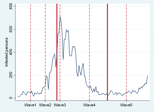
COVID-19 infection rates in Japan and survey waves. Note: The graph depicts the cross-wave development of the daily numbers of persons getting infected with COVID-19 in Japan, evaluated by the daily numbers of persons who are in the positive PCR test. The first, second, third, fourth and fifth waves were conducted on March 13–16, March 27–30, April 10–13, May 8–11, and June 12–15, respectively. Dashed lines indicate the date of the surveys. Two bold lines show the dates when the state of emergency was declared (April 7), and when the state of emergency was deregulated (May 25).
COVID-19 infection rates in Japan and survey waves. Note: The graph depicts the cross-wave development of the daily numbers of persons getting infected with COVID-19 in Japan, evaluated by the daily numbers of persons who are in the positive PCR test. The first, second, third, fourth and fifth waves were conducted on March 13–16, March 27–30, April 10–13, May 8–11, and June 12–15, respectively. Dashed lines indicate the date of the surveys. Two bold lines show the dates when the state of emergency was declared (April 7), and when the state of emergency was deregulated (May 25).
Summary of the survey waves
| Survey wave | Survey dates | Numbers of responses | Response rates | Numbers in balanced panel |
|---|---|---|---|---|
| 1st | 2020/03/13–03/16 | 4,359 | 54.70% | 2,894 |
| 2nd | 2020/03/27–03/30 | 3,495 | 80.20% | 2,894 |
| 3rd | 2020/04/10–04/13 | 4,013 | 92.20% | 2,894 |
| 4th | 2020/05/08–05/11 | 3,996 | 91.90% | 2,894 |
| 5th | 2020/06/12–06/15 | 3,877 | 89.40% | 2,894 |
| Total | 19,740 | 14,470 |
Based on the Act on Special Measures against Pandemic Influenza, Japan’s prime minister declared a state of emergency on April 7 for seven large prefectures, including Tokyo and Osaka, to control the pandemic. Although the declaration had no legal force in regulating people’s activities, the seven prefectures were requested to follow the guideline of activities in the private and public sectors. This significantly affected the whole Japanese society and economy. Soon after the declaration of a state of emergency, the third wave was conducted from April 10 to 13, with 4,013 participants. We conducted the fourth wave from May 8 to 11 with 3,996 participants. By that time, the daily infection rate had begun declining, while the state of emergency was extended until the end of May. After the state of emergency was deregulated on May 25, the fifth wave was conducted on June 12 to 15 with 3,877 participants, when society began attempting to return to normalcy, that is, the situation before the pandemic.
As Table 1 shows, a total of 2,894 people participated in all five waves. In the analysis in the following sections, although the results would not change even if we used the whole, unbalanced sample, we focus on this subset of observations constituting a balanced panel sample.
2.2 Risk Attitude
In the survey, two hypothetical questions, Q1 and Q2, are used to evaluate participants’ risk attitudes in the loss domain. They are asked to choose the highest acceptable insurance premium from a given multiple price list, to cover a probabilistic risk of losing a certain amount of money. In Q1, participants are assumed to lose an amount of JPY 1,00,000 (approximately USD 1,000) with a 50% probability, whereas they are supposed to lose JPY 5 million (approximately USD 50,000) with a probability of 0.1% (for the precise question in the survey, see Online Appendix B1) in Q2.
Note that Q1 and Q2 are designed such that they differ in the skewness of the probability distribution of negative outcomes. In Q1, the outcome of losing JPY 0 or JPY 100,000 occurs with a fifty-fifty chance, implying that the distribution has zero skewness. In contrast, participants are supposed to lose a huge amount of money (JPY 5 million) with a small probability (0.1%) in Q2, in which case, skewness is highly negative (–31.575).4 As prospect theory shows, people with an inverse S-shaped probability weighting function tend to be averse to probabilistic losses with a negatively skewed distribution; they are pessimistic about rare negative events.5 By examining the responses to both questions with different skewness, we can clearly characterize the participants’ risk attitudes by means of the value and probability weighting functions.
We suppose that each participant responds to Q1 and Q2 by evaluating the (negative) value of the corresponding probabilistic losses based on their prospect theory values V1 and V2. We let xi (i = 1, 2) denote the negative outcome of question Qi (x1 = –100, 000; and x2 = –5, 000, 000) and pi, the probability that xi occurs (p1 = 0.5; and p2 = 0.001). Accordingly, the prospect theory value of the probabilistic loss supposed in question Qi is evaluated using the value function v(xi), which evaluates the subjective value of outcome xi, and the probability weighting function w(pi), which represents the subjective impact of probability pi, as:6
Following the functional specification of the two functions in Tversky and Kahneman (1992), we specify functions v (x) and w (p) in the loss domain (x < 0). Letting α (0 ≤ α ≤ 1) denote the power parameter of the value function in the loss domain, which determines the degree of risk-lovingness (1 – α), and λ represent a parameter that determines the degree of loss aversion, the value function a la Tversky and Kahneman (1992) is given as
With δ (0 ≤ δ ≤ 1) denoting a parameter for the probability weighting function, where (1 – δ) determines the depth of the resulting inverse S-shaped curve, the probability weighting function w (p) is given by
Note that, irrespective of specification (2) of the value function, the participants’ choices in this study do not depend on loss aversion parameter λ, because it does not consider prospects in which negative and positive outcomes are mixed.
Let Ri (i = 1, 2) be the highest acceptable insurance premium revealed from the response data to question Qi (see Online Appendix B2). By construction, the prospect-theory values are equalized between paying Ri and taking a risk of negative prospect (xipi; 0, 1 – pi):
where λ disappears, because it is canceled out.
By solving these simultaneous equations, we can obtain the values of α and δ for each participant. By taking the natural log of the equations and rearranging the results, we have the following two equations:
Regarding the values of the highest acceptable insurance premiums R1 and R2 that each participant revealed in Q1 and Q2, the value of parameter δ in the probability weighting function is obtained from (6) for each respondent. Consequently, the value of parameter α for the value function is computed from (7) for each participant given the value of δ.7
3 Results
3.1 Mean Comparison
Table 2 summarizes the cross-wave changes in the participants’ acceptable insurance premiums (R1, R2) in questions Q1 and Q2, and the risk premiums implied therefrom, R1/50, 000 – 1 for Q1 and R2/5, 000 – 1 for Q2. Note that a positive risk premium implies risk-averse behavior, whereas a negative one implies a risk-loving choice. Table 2 clearly shows two distinct tendencies. First, participants are consistently risk-loving for Q1, and risk-averse for Q2 through all five waves. This is consistent with the prospect theory’s prediction that people are risk-loving when evaluating a prospect defined over the loss domain, insofar as the payoff probability distribution is insignificantly negatively skewed, as in Q1. The same theory states that people are risk averse in the loss domain when the associated distribution is significantly negatively skewed, as in Q2.
Summary statistics of insurance premimums gathered from Questions Q1 and Q2.
| Question | Q1 | Q2 | |||||||
|---|---|---|---|---|---|---|---|---|---|
| Insurance covering: Skewness | (–JPY100,000, 0.5) zero | (–JPY5,000,000, 0.001) highly negative (–31.575) | |||||||
| Acceptable premium (JPY R1) | Implied risk premium (R1/50,000-1) | Acceptable premium (JPY R2) | Implied risk premium (R2/5,000-1) | ||||||
| Mean | S.D. | Mean | S.D. | Mean | S.D. | Mean | S.D. | Obs. | |
| Wave 1 | 7,999.128 | 11,456.750 | –0.840 | 0.229 | 19,157.170 | 91,401.650 | 2.831 | 18.280 | 2,894 |
| Wave 2 | 7,143.150 | 10,405.030 | –0.857 | 0.208 | 15,602.410 | 86,706.680 | 2.120 | 17.341 | 2,894 |
| Wave 3 | 5,252.021 | 9,234.972 | –0.895 | 0.185 | 8,789.115 | 47,888.520 | 0.758 | 9.578 | 2,894 |
| Wave 4 | 5,194.186 | 9,147.053 | –0.896 | 0.183 | 10,216.000 | 62,442.170 | 1.043 | 12.488 | 2,894 |
| Wave 5 | 4,805.805 | 8,763.868 | –0.904 | 0.175 | 9,011.869 | 60,912.300 | 0.802 | 12.182 | 2,894 |
| All | 6,078.858 | 9,930.297 | –0.878 | 0.199 | 12,555.310 | 71,906.760 | 1.511 | 14.381 | 14,470 |
Second, and more importantly, Table 2 shows that as the wave proceeds and COVID-19 spreads, risk premiums implied from Q1 and Q2 decrease almost monotonically. This implies that average participants become more risk-loving in Q1 and less risk averse in Q2 as the pandemic spreads.
Our main interest is in how these behavioral tendencies that occur with the spread of COVID-19 are quantified in terms of risk preference parameters in prospect theory. Table 3, which shows the summary statistics for the elicited values of prospect theory parameters α and δ in each wave, presents three noteworthy points. First, the mean values of α and δ are both between 0 and 1 in each wave. This implies that the value function and probability weighting function elicited, on average, have a diminishing sensitivity property that prospect theory predicts. In other words, the average participant has a convex value function in the loss domain, displaying diminishing sensitivity to marginal increases in the loss amount. The probability weighting function in the loss domain of average participants is inversely S-shaped; therefore, it has the diminishing sensitivity property. Overweighting occurs for tail loss risks, whereas underweighting takes place for non-tail loss risks.
Summary statistics of prospect-theory paramters in the loss domain.
| α | δ | ||||
|---|---|---|---|---|---|
| Mean (S.D.) | H0: Wave t = Wave t – 1 | Mean (S.D.) | H0: Wave t = Wave t – 1 | Obs. | |
| Wave 1 | 0.458 | n.a. | 0.424 | n.a. | 2,894 |
| (0.223) | (0.131) | ||||
| Wave 2 | 0.438 | 0.001 | 0.417 | 0.023 | 2,894 |
| (0.206) | (0.113) | ||||
| Wave 3 | 0.398 | 0.000 | 0.400 | 0.000 | 2,894 |
| (0.171) | (0.109) | ||||
| Wave 4 | 0.397 | 0.823 | 0.399 | 0.765 | 2,894 |
| (0.177) | (0.107) | ||||
| Wave 5 | 0.387 | 0.034 | 0.394 | 0.089 | 2,894 |
| (0.170) | (0.101) | ||||
| All | 0.416 | 0.407 | 14,470 | ||
| (0.192) | (0.113) | ||||
Second, the mean values of α and δ seem to monotonically decrease as the wave proceeds, suggesting that diminishing sensitivity tends to be stronger for both the value and probability weighting functions. Figure 2(a) and (b) depict the elicited mean cross-wave shifts of both functions. With COVID-19 spreading, the value function becomes more curved, and the inverse S shape of the probability weighting function becomes deeper. Particularly, the effects occur most substantially between Waves 2 and 3, that is, in response to the declaration of the state of emergency.
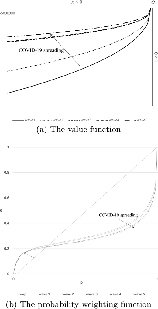
Cross-wave shifting of the value and the probability weighting functions in the loss domain. Note: The figures depict the cross-wave shifting of the value function ([a]) and the probability weighting function ([b[), where both are defined over the loss domain. The loci of the functions are computed using mean values of α and δ at each wave summarized in Table 4. Regarding the value function, we set the loss aversion parameter λ = 2.25, the median value obtained by Tversky and Kahneman (1992).
Cross-wave shifting of the value and the probability weighting functions in the loss domain. Note: The figures depict the cross-wave shifting of the value function ([a]) and the probability weighting function ([b[), where both are defined over the loss domain. The loci of the functions are computed using mean values of α and δ at each wave summarized in Table 4. Regarding the value function, we set the loss aversion parameter λ = 2.25, the median value obtained by Tversky and Kahneman (1992).
Figure 3(a) and (b) show the statistical significance of these preference shifts, where comparisons are made for the male and female samples. For either of the male or female sample, α and δ both exhibit the sharpest, statistically significant declines in the third wave. As the third wave was conducted shortly after the government declared the state of emergency, the largest reductions in the risk parameters could reflect the direct and indirect effects of the declaration. Except for significant reductions in the female participants’ α in the second wave, other decreases in α and δ between two consecutive waves are statistically insignificant. It is important to note, however, that these results are based on simple mean comparison, without controlling for fixed effects. With fixed effects being controlled, cross-wave differences and, consequently, the effects of the outbreak of COVID-19 become more significant, as we show in the next section.
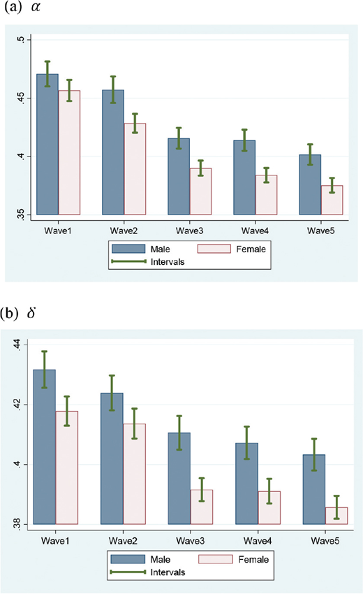
Cross-wave comparison of prospect theory parameters in the loss domain: Balanced panel. Note: The balanced panel data are used (N=14,470). Parameters α and δ represent the value and probability weighting functions, respectively. The first, second, third, fourth and fifth waves were conducted on March 13–16, March 27–30, April 10–13, May 8–11, and June 12–15, respectively. The intervals represent the 95% confidence intervals.
Cross-wave comparison of prospect theory parameters in the loss domain: Balanced panel. Note: The balanced panel data are used (N=14,470). Parameters α and δ represent the value and probability weighting functions, respectively. The first, second, third, fourth and fifth waves were conducted on March 13–16, March 27–30, April 10–13, May 8–11, and June 12–15, respectively. The intervals represent the 95% confidence intervals.
We can also find gender differences in Figure 3(a) and (b). Both α and δ are lower for females than males, implying that the females tend to exhibit a stronger diminishing sensitivity for both prospect-theory functions. This result is consistent with that of Fehr-Duda et al. (2006), who showed through laboratory experiments, that women’s elicited probability weighting function tends to be more curved than men’s in either the gain or loss domain. Particularly, as in this study, the study detected the same tendency in the context of insurance evaluation. Our findings are consistent with these results.89
Our finding that females’ degree of risk-lovingness in the loss domain is larger than that of males seems to contradict the stylized tendency that the former is more risk averse than the latter (e.g., Croson and Gneezy, 2009). However, previous research does not control for possible gender differences in probability weighting. After controlling for gender difference in probability weighting, Fehr-Duda et al. (2006) found no cross-gender difference in the degree of risk-lovingness with respect to the value function. Both their results and ours suggest that gender differences in risk aversion could differ from what the previous literature claimed.
3.2 Regressions
By controlling for the effects of individual participants’ heterogeneous attributes, that is, fixed effects, we confirm the validity of the finding in the previous subsection regarding the shifting of risk attitudes during the COVID-19 pandemic. Accordingly, we estimate two fixed effect models for prospecttheory parameters α and δ using the balanced panel data.10 First, the two risk parameters are regressed on variable Infected COVID 19, the rate of persons infected with COVID-19 in each respondent’s residential prefecture at each wave. In the second model, we add four-wave dummy variables for the 2nd to 5th waves, Wave2-Wave5, to the set of regressors, where Wave 1 is the reference case, to capture nationwide cross-wave effects of the pandemic.
Table 4 summarizes the estimation results, which show the shifting of the risk parameters in two ways. First, Panel A shows that, in either the male, female, or full sample, both risk parameters α and δ are negatively associated with Infected COVID 19. This implies that the respondents’ diminishing sensitivities 1 – α and 1 – δ are both positively associated with the rate of persons infected with COVID-19 in their residence prefectures.
Fixed effect model estimations: Balanced panel.
| Panel A | ||||||
|---|---|---|---|---|---|---|
| Dep. Variable = α | Dep. Variable = δ | |||||
| Full | Male | Female | Full | Male | Female | |
| Infected COVID 19 | –2.401** | –2.416** | –2.385** | –0.996** | –0.947** | –1.046** |
| (0.154) | (0.254) | (0.174) | (0.092) | (0.137) | (0.123) | |
| Within R-Sq. | 0.02 | 0.02 | 0.03 | 0.01 | 0.01 | 0.01 |
| Groups | 2,894 | 1,458 | 1,436 | 2,894 | 1,458 | 1,436 |
| Obs. | 14,470 | 7,290 | 7,180 | 14,470 | 7,290 | 7,180 |
| Panel B | ||||||
| Dep. Variable = α | Dep. Variable = δ | |||||
| Full | Male | Female | Full | Male | Female | |
| Infected COVID 19 | –0.267 | –0.603 | 0.089 | 0.008 | –0.010 | 0.028 |
| (0.247) | (0.412) | (0.263) | (0.135) | (0.193) | (0.188) | |
| Wave1 | <default> | <default> | ||||
| Wave2 | –0.019** | –0.014* | –0.025** | –0.007** | –0.008* | –0.006 |
| (0.004) | (0.007) | (0.005) | (0.003) | (0.003) | (0.003) | |
| Wave3 | –0.059** | –0.052** | –0.065** | –0.025** | –0.021** | –0.029** |
| (0.004) | (0.006) | (0.005) | (0.003) | (0.004) | (0.003) | |
| Wave4 | –0.058** | –0.046** | –0.069** | –0.026** | –0.024** | –0.028** |
| (0.004) | (0.008) | (0.006) | (0.003) | (0.004) | (0.004) | |
| Wave5 | –0.067** | –0.058** | –0.076** | –0.030** | –0.029** | –0.032** |
| (0.005) | (0.008) | (0.007) | (0.003) | (0.004) | (0.004) | |
| Waves 2 vs 3 | P = 0.00 | P = 0.00 | P = 0.00 | P = 0.00 | P = 0.00 | P = 0.00 |
| Waves 3 vs 4 | P = 0.73 | P = 0.35 | P = 0.68 | P = 0.68 | P = 0.41 | P = 0.71 |
| Waves 4 vs 5 | P = 0.00 | P = 0.00 | P = 0.00 | P = 0.00 | P = 0.04 | P = 0.07 |
| Within R-Sq. | 0.05 | 0.03 | 0.08 | 0.03 | 0.02 | 0.04 |
| Groups | 2,894 | 1,458 | 1,436 | 2,894 | 1,458 | 1,436 |
| Obs. | 14,470 | 7,290 | 7,180 | 14,470 | 7,290 | 7,180 |
Note: Parameters α and δ represent the value function and the probability weighting function, respectively, in the loss domain (see equations [2] and [3]), where a higher a implies a lower degree of risk-lovingness, and where a smaller δ value implies a deeper inverse S shape of the probability weighting function. Panel A represents the results of fixed effect model estimation with the rate of persons infected with COVID-19 in each respondent’s residence prefecture at each wave being introduced as unique regressor. Panel B shows the estimation result when four wave dummies are added as regressors. Numbers within parentheses are robust standard errors clustered on individuals. ** and * indicate statistical significance at 1% and 5% levels, respectively.
Second, in Panel B, where α and δ are regressed on wave dummies and Infected COVID 19, the significant upward shifting of the respondents’ diminishing sensitivity 1 – α and 1 – δ are captured by negative coefficients of the wave dummy variables, rather than those of Infected COVID 19. This implies that the observed effects on people’s risk attitudes represent the nationwide, total influence of the pandemic, including deteriorations in various economic and social conditions, rather than the pure direct effect of local virus infection risk. To be consistent with this interpretation, Boutin et al. (2022) shows that the COVID-19 pandemic affected risk preferences in the gain and loss domains though effects on emotional concerns, rather than through actual effects in individual daily life around small neighborhoods.
The effects occur most significantly in Wave 3, that is, just after the declaration of the state of emergency significantly affected the entire Japanese society and economy. The coefficients of Wave3 in absolute value are almost more than triple those of Wave2.11 Additionally, unlike the simple t-tests in Figure 3, the estimation in Panel B shows that marginal reductions in α and δ between two consecutive waves are significant, except for those between Waves 3 and 4. This means that 1 – α and 1 – δ continue to rise, that is, diminishing sensitivity is monotonically enhanced for the value and the probability weighting functions in association with the spread of COVID-19.
Enhanced diminishing sensitivity in two prospect-theory functions has different implications for the effect of the pandemic on risk attitudes. With the value function exhibiting stronger diminishing sensitivity, that is, with (1 – α) continuously increasing, people gradually become less sensitive to an increase in losses, and consequently feel less displeasure from given losses. For example, for average participants in Wave 5, the displeasure of losing JPY 5 million, evaluated by |v (JPY 5 million)|12 is only 0.33 times that of Wave 1.
Note that such a reduction in feeling displeasure |v (x)| against a loss x(< 0) owing to an increase in (1 – α) becomes larger as the loss amount |x| increases. Therefore, in association with the spread of COVID-19, people feel less displeasure from large losses (e.g., losing JPY 5 million) at a higher speed than they do with smaller losses (e.g., losing JPY 1000). Therefore, they become less cautious about large losses, for example, suffering serious diseases, relative to smaller ones, for example, paying small costs for disease protection.13
As the probability weighting function enhances its diminishing sensitivity property during the pandemic, the overweighting of tail losses and underweighting of non-tail losses become more robust. For example, the probability weight that average participants put on a negative outcome occurring with probability 0.1%, that is, w(0.1%), becomes larger from 4.7% in Wave 1 to 5.6% in wave 5, implying that overweighting becomes more robust. In contrast, the probability weight w(50%) decreases from 29.1% in Wave 1 to 26.3% in Wave 5.14 In other words, underweighting for non-tail losses is enhanced during the spread of the pandemic.
In sum, COVID-19 affects people’s risk attitudes in two ways. First, owing to the pandemic, people become less sensitive to an increase in losses, particularly when they are large. Second, people become more pessimistic about tail loss risks, and more optimistic about non-tail loss risks. The two findings imply that people are the least sensitive to a large non-tail loss risk. Policy-makers should consider this side effect as the risk of large non-tail losses is widely prevalent (e.g., risk of virus infection when staying home with infected family members, risk of developing cancer when smoking, risk of global warming, etc.), which could weaken people’s preventive and/or precautionary behavior against large risks.
These results relate to the existing literature in the following ways. First, the result that the degree of risk-lovingness in the loss domain continuously rose with the spread of the pandemic appears to differ from the empirical results in the literature, which states that negative shocks, either disasters or stressful events, enhance risk aversion (Page et al., 2014; Kandasamy et al., 2014; Cameron and Shah, 2015; Casser, et al., 2017; Bu et al., 2020; Di Falco and Vieider, 2022). However, these studies, except Kandasamy et al. (2014), do not control for the effect on probability weighting. More importantly, previous studies evaluate risk aversion in the gain domain, while this study considers the loss domain. Although the results may differ with respect to the effects on the degree of risk aversion, it could be reconciled if we interpret the results in terms of diminishing sensitivity. The findings of previous studies and those of this study commonly indicate that pandemics and other negative shocks reinforce diminishing sensitivity to a marginal increase in losses and gains. The reflection effect, in which risk preferences in the gain domain are the mirror image of those in the loss domain, is considered robust (Kahneman and Tversky, 1979; Fehr-Duda et al., 2006; Abdellaoui et al., 2007; Dhami, 2016). This interpretation is considered to have certain validity.
Second, Li et al. (2011) and Page et al. (2014) show that natural disasters lead people to display stronger preferences for prospects with positively skewed prizes. They attribute this to the increased overweighting of small probabilities. However, they do not estimate the probability weights or control for the effect on the value function. Our finding that people’s probability weighting exhibits stronger diminishing sensitivity during the pandemic provides evidence for their claim.
4 Discussions
4.1 Possible Mechanisms
We could consider two mechanisms, mental stress and liquidity shortage, in which the spread of the COVID-19 pandemic affected participants’ risk attitude.
4.1.1 Mental Stress
The spread of the COVID-19 infection directly or indirectly significantly negatively affected mental health. For example, Yamamoto et al. (2020) reported that 33.6% of 11,333 participants experienced mild-to-moderate psychological distress, and 11.5% suffered from serious mental distress. Mental stress is known to affect risk attitude (Haushofer and Fehr, 2014; Cohn et al., 2015; Cahli kovai and Cingl, 2017). Therefore, mental stress induced by the COVID-19 pandemic could affect people’s risk attitudes. Our results could be interpreted as reflecting the influence of mental stress caused by COVID-19.
In this sense, our results are comparable with the findings of Kandasamy et al. (2014), who gave participants a dose of hydrocortisone and examined how experimentally raised stress hormone (cortisol) levels affected their risk attitudes. The findings were captured by the shapes of the value and probability weighting functions. The authors show that experimentally raised cortisol levels (i) made the participants’ value function in the gain domain more concave, wherein they became more risk averse in the gain region, and (ii) deepened the inverse S shape of the weighting probability function for male participants. In other words, overweighting of positive tail outcomes and underweighting of positive non-tail outcomes were more exaggerated under increased stress for males. If our result reflects the stress effect of the pandemic, our finding on its effect on the probability weighting function is consistent with, and even stronger, than that of Kandasamy et al. (2014) as stated in (ii), in which the same effect was not detected in the female sample.15 Moreover, our finding relates to Kandasamy et al.’s (2014) result (i); both commonly indicate that stressful events enhance the diminishing sensitivity of the value function.
4.1.2 Liquidity Shortage
As COVID-19 had a persistent negative income effect,16 another plausible mechanism could be the lack of liquidity; under a liquidity shortage, participants might become more reluctant to buy insurance as negative income shocks continue (McDermott et al., 2014), which could result in reductions in acceptable risk premiums in Q1 and Q2. To examine the validity of this hypothesis, we re-estimate the fixed effect model by adding to the set of independent variables the product terms of wave dummies and a low income dummy, which equal one when the participant belongs to the bottom 10% income class at Wave 1, and zero otherwise.17 If the lack-of-liquidity hypothesis holds, the coefficients of the product terms are negative.
As seen in Table 5, the hypothesis is invalid. Contrary to the prediction of the hypothesis, the coefficients of the interaction terms of wave dummies and the low income group indicator are all positive and highly significant, especially for the α estimation. This result could indicate the rational riskinsuring behavior of low-income participants. Relative to those in higher income groups, they became more willing to buy insurance in Q1 and Q2 because of poor self-insurance ability during the pandemic.
Fixed effect model with interaction terms with a low-income group indicator.
| Dep. Variable = α | Dep. Variable = δ | |||||
|---|---|---|---|---|---|---|
| Full | Male | Female | Full | Male | Female | |
| Wave2 × | 0.021 | 0.029 | 0.013 | 0.003 | 0.001 | 0.005 |
| Bottom 10% | (0.011) | (0.019) | (0.012) | (0.006) | (0.001) | (0.009) |
| Wave3 × | 0.027** | 0.015 | 0.038** | 0.005 | –0.005 | 0.016* |
| Bottom 10% | (0.008) | (0.013) | (0.01) | (0.006) | (0.01) | (0.008) |
| Wave4 × | 0.024** | 0.019 | 0.028* | 0.012 | 0.012 | 0.011 |
| Bottom 10% | (0.008) | (0.013) | (0.011) | (0.006) | (0.009) | (0.008) |
| Wave5 × | 0.031** | 0.029* | 0.033** | 0.019** | 0.021* | 0.018* |
| Bottom 10% | (0.009) | (0.013) | (0.012) | (0.007) | (0.01) | (0.009) |
| Wave1 | <default> | <default> | ||||
| Wave2 | –0.022** | –0.017** | –0.027** | –0.008** | –0.008* | –0.007 |
| (0.004) | (0.007) | (0.006) | (0.003) | (0.004) | (0.004) | |
| Wave3 | –0.062** | –0.054** | –0.069** | –0.025** | –0.020** | –0.030** |
| (0.004) | (0.007) | (0.006) | (0.003) | (0.004) | (0.003) | |
| Wave4 | –0.060** | –0.048** | –0.073** | –0.027** | –0.025** | –0.029** |
| Wave4 | (0.005) | (0.008) | (0.007) | (0.003) | (0.004) | (0.004) |
| Wave5 | –0.070** | –0.062** | –0.079** | –0.033** | –0.032** | –0.034** |
| Wave5 | (0.006) | (0.009) | (0.007) | (0.003) | (0.004) | (0.004) |
| Within R-Sq. | 0.05 | 0.04 | 0.08 | 0.03 | 0.02 | 0.04 |
| Groups | 2,894 | 1,458 | 1,436 | ,894 | 1,458 | 1,436 |
| Obs. | 14,470 | 7,290 | 7,180 | 14,470 | 7,290 | 7,180 |
Note: Bottom 10% represents a binary indicator which equals one when the participant’s household belongs to the bottom 10% income group in Wave 1, where income data are not available for the other waves. Although its result is not reported, the rate of persons infected with COVID-19 in each respondent’s residence prefecture in each wave is included as a control variable. Numbers within parentheses are robust standard errors clustered on individuals. ** and * indicate statistical significance at 1% and 5% levels, respectively.
4.2 Comparing Risk Preference Before and After COVID-19
We have interpreted that the observed changes in the α and δ values observed during the pandemic period reflect some level of effect, direct or indirect, of the pandemic. However, the finding would be weak, because the elicited parameter values are based on the data after the outbreak of the pandemic and not compared with those before the pandemic.
To address this limitation, we can use comparable data from the NTT Human Information Data 2018 (NTTHID2018, hereafter), a large-scale internet survey conducted in Japan by the NTT Human Information Research Institute, Inc. in October 2018 (N=20,160). Participants were selected from adults in Japan using the stratified assignment method, as in our survey. In the NTT survey, one of the authors participated in designing the questionnaire, and asked participants questions similar to Q1 and Q2, where hypothetical loss amounts were JPY 10,000, rather than JPY 100,000 in Q1, and JPY 50,000 rather than JPY 5 million in Q2. The probability setting is similar to that in Q1 and Q2. As participants were selected in a similar way as in this panel survey, a comparison of the elicited risk attitude between the NTTHID2018 sample and that of the present panel data could provide certain information on how people’s risk attitudes differ between the pre- and post-outbreak periods of the pandemic. If our conclusion that the pandemic enhances diminishing sensitivity for prospect-theory risk preference is supported, diminishing sensitivity in the pre-COVID-19 period, elicited from the NTTHID2018 sample, will be weaker than it is in the present panel data. This prediction will hold valid especially for the Wave 1 sample, in which diminishing sensitivity is the weakest among the five wave samples.
To compare risk parameters before and after the outbreak of the pandemic, we compute both simple sample and weighted means of the risk parameters. The weights are calculated to conform the gender-age-residential prefecture distributions of the two samples to the census distribution derived from Population Estimates in 2019, and Comprehensive Survey of Living Condition in 2018. Therefore, the weighted means could be considered the means of the representing sample of Japan, corrected for possible sampling biases.
Table 6 compares the mean values for α and δ between the Wave 1 sample of the present panel data, and the pre-COVID-19 sample of NTTHID2018, where the first, and second rows represent simple sample means and weighted means, respectively. For both male and female samples, and for both (unweighted) simple and weighted means, the pre-COVID-19 mean values of α and δ are significantly larger than the corresponding post-COVID-19 values, that is, the Wave 1 mean values. This could be considered the indirect evidence that the observed cross-wave increase in diminishing sensitivity for prospect-theory risk preferences reflect the effect of the COVID-19 pandemic.
Comparing risk preference before and after COVID-19.
| α | |||||
|---|---|---|---|---|---|
| Male | Female | Census-data weights | |||
| Wave 1 | NTTHID2018 | Wave 1 | NTTHID2018 | ||
| Mean | 0.465 | 0.618 | 0.450 | 0.566 | |
| (S.D.) | (0.241) | (0.283) | (0.204) | (0.262) | |
| t-value | 22.134 | 19.427 | No | ||
| obs. | 1,458 | 10,365 | 1,436 | 9,591 | |
| Mean | 0.474 | 0.624 | 0.456 | 0.578 | |
| (S.D.) | (0.332) | (0.364) | (0.261) | (0.490) | |
| t-value | 14.634 | 9.177 | Yes | ||
| obs. | 1,458 | 7,741 | 1,436 | 6,641 | |
| δ | |||||
| Male | Female | Census-data weights | |||
| Wave 1 | NTTHID2018 | Wave 1 | NTTHID2018 | ||
| Mean | 0.431 | 0.501 | 0.417 | 0.447 | |
| (S.D.) | (0.144) | (0.204) | (0.117) | (0.169) | |
| t-value | 16.269 | 8.093 | No | ||
| obs. | 1,458 | 10,365 | 1,436 | 9,591 | |
| Mean | 0.438 | 0.502 | 0.422 | 0.449 | |
| (S.D.) | (0.240) | (0.246) | (0.176) | (0.305) | |
| t-value | 9.092 | 3.239 | Yes | ||
| obs. | 1,458 | 7741 | 1436 | 6641 | |
Additionally, the table shows that females’ α and δ are also on average smaller than males’ in the NTTHID2018 sample, implying that females exhibit stronger diminishing sensitivity than males in the loss domain, consistent with the gender difference found in Figure 3.
4.3 Alternative Estimation
Using the maximum likelihood method, we re-estimate the system for our prospect-theory model. This has two merits. First, it enables us to estimate the two risk parameters for the representative participant, and consequently check the robustness of our finding, which states that diminishing sensitivity becomes more robust during the pandemic.
As the second merit, we can check the model fitting of the prospect theory model. Thus far, we have assumed a priori the prospect theory model, formalized by (1) to (3). We check whether the prospect theory model has a better fit to the observed data than the usual one-parametric expected value model, in which people respond to questions Qi (i = 1, 2) based on the expected value of the value function,
instead of (1).
We therefore estimate two systems: one for the prospect theory model, comprising (4) and (5), and the other for the expected value model (8), which is rewritten by replacing probability weights w(0.5) and w(0.001) in (4) and (5) with objective probability values 0.5 and 0.001 as:
Note that the expected value model, comprising (9) and (10), is a special case of the prospect theory model with restriction that δ = 1. The prospect theory model therefore nests the expected value model.
The goodness of fit is compared between the two models in three ways. We first test the nested hypothesis using Wald test to check if δ = 1 in the prospect theory model. However, because of the nonlinearity of the models, various tests including Wald test possibly report inconsistent results. Therefore, we also compare the fit of the two models using log-likelihood ratio test and AIC.
Using the full information maximum likelihood method, we estimate the logarithmic version of each system, where four wave dummies, Wave2 to Wave5, are added to each preference parameter.
Table 7 summarizes the results. It is important to note the following two points. First, the regression result shows that the two prospect-theory parameters tend to decline during the sample period, similar to that in Tables 2 and 3. This confirms our main result that diminishing sensitivity becomes more robust during the pandemic.
Prospect theory model vs. expected value model
| Prospect theory model Expected value model | |||
|---|---|---|---|
| α | δ | α | |
| 0.387** | 0.392** | 1.305** | |
| (0.002) | (0.001) | (0.007) | |
| Wave2 | –0.009** | –0.003 | –0.017* |
| (0.003) | (0.002) | (0.008) | |
| Wave3 | –0.037** | –0.016** | –0.034** |
| (0.003) | (0.002) | (0.008) | |
| Wave4 | –0.038** | –0.017** | –0.036** |
| (0.003) | (0.002) | (0.008) | |
| Wave5 | –0.045** | –0.020** | –0.040** |
| (0.003) | (0.002) | (0.008) | |
| Log-likelihood | –2,70,809.8 | –283,371.3 | |
| Obs. | 14,470 | 14,470 | |
| (1) Wald test (δ = 1 for all waves) | |||
| χ2 | 1,411,966** | ||
| (2) Log-likelihood ratio test | |||
| χ2 | 25,123.0** | ||
| (3) AIC | 37.432 | 39.167 | |
Note: The system equation of the prospect theory model, defined by (4) and (5), and that of the expected value model, comprising (9) and (10), are estimated from the balanced panel dataset using the full information maximum likelihood method. The rows of Wave2 to Wave5 show the coefficients of the corresponding dummy variables, with the Wave 1 value being the reference. Numbers within parentheses are standard errors. Rows (1) through (3) represent the goodness-of-fit statistics. Row (1) shows the result of Wald test with the null hypothesis that in the prospect theory model, the probability weights equal objective probabilities for all waves: δ = 1, as is the case of the expected value model. Row (2) represents the result of log-likelihood ratio test for the relative goodness-of-fit of the prospect theory model to the expected value model. Row (3) compares the values of the Akaike information criterion. ** and * indicate the statistical significance at 1% and 5% levels, respectively.
Second, Table 7 shows that the prospect theory model better fits to our data than the one-parametric expected value model: (1) the Wald test strongly rejects the null hypothesis that δ = 1; (2) the χ2-value of the log-likelihood ratio test is 25,123.0, which strongly rejects the equality of the log-likelihood values between the two models; and (3) the AIC value for the prospect theory model (37.432) is smaller than that for the expected value model (39.167). Therefore, the fit of the prospect theory specification is better to our data, than the one-parametric expected value specification with any statistics, even when correcting for the difference in the number of parameters. This reflects the fact that the usual expected value specification cannot explain why people’s risk attitude can be either risk-averse or risk-loving, depending on the skewness of the probability distribution, as observed in our samples.
These results can be shown robust against controlling for the effects of (i) the rate of persons infected with COVID-19 in each respondent’s residential prefecture, (ii) the gender difference, and (iii) alternative function forms of the expected value model (e.g., CARA, instead of the present CRRA form).
4.4 Implications for the Stability of Risk Preferences
Our panel study has implications for the stability of risk preferences. As surveyed by Chuang and Schechter (2015), many researchers have been examining how stable risk and other preferences evaluated using experiments and surveys are over time, across different questions/tasks, between incentivized and hypothetical settings, etc. The discussions still remain controversial. Particularly, based on their unique panel data in Paraguay, Chuang and Schechter show that estimated game-based measures of risk preferences tend to be very noisy, in that the measured risk preferences are not stable over time or across games, namely across frames of questions and tasks, nor affected by negative income/health shocks.
Irrespective of their claim, our dataset implies that participants’ risk choices and their imputed risk preferences are quite stable. First, as shown in Online Appendix C, significant positive cross-wave correlations are found both in acceptable insurance premiums R1 and R2 for Q1 and Q2, and in the imputed prospect theory risk parameters α and δ. The mean cross-wave correlation coefficient amounts to 0.549 for R1 and 0.282 for R2. Imputed value function parameter α has cross-wave correlation of 0.515 on average. Regarding probability weighting function parameter δ, the mean cross-wave correlation amounts to 0.500 (for details, see Table A2 in Online Appendix C). Second, imputed risk attitudes are also consistent between acceptable insurance premiums R1 and R2, namely between underlying survey questions Q1 and Q2. As shown in Table A3 in the Online Appendix, the crossquestion correlations for acceptable insurance premiums are between 0.370–0.413. Finally, as we have shown in the previous sections, negative shocks owing to COVID-19 systematically affected participants’ risk attitudes and the imputed risk preferences. These findings imply that, in contrast to what is emphasized by Chuang and Schechter (2015), measured risk attitudes in our survey are quite stable.
5 Conclusions
Based on the analysis of a unique five-wave panel survey in Japan, we find that diminishing sensitivity in the loss domain became more robust for people’s prospect-theory risk preference with the spread of COVID-19. Therefore, (i) losses, particularly large losses, became less displeasing, and (ii) people became more pessimistic toward tail loss risks, but more optimistic toward non-tail loss risks.
This research provides new insights in understanding the effects of pandemics and other negative shocks on risk attitudes. First, the effects are captured in terms of resulting changes in diminishing sensitivity, rather than in risk aversion/tolerance. Our findings and those of the literature commonly indicate that pandemics and other negative shocks enhance diminishing sensitivity in risk evaluation. Second, by detecting the distorting effect of the pandemic on probability weighting, we provide robust empirical evidence to the previous finding, stating that disasters drive those affected to avoid tail loss risks (Li et al., 2011; Page et al., 2014). Our finding on this point could also be considered evidence to Bu et al.’s (2020) conjecture that changes in people’s risk attitudes after the outbreak could occur because of their pessimistic beliefs on various probabilistic environments.
Findings (i) and (ii) imply that, after pandemic outbreaks and other negative shocks, people become much less cautious to the risk of non-tail, large losses. Because the risk of large non-tail losses is widely prevalent (e.g., the risk of virus infection when joining a meeting/party, risk of developing cancer when smoking, risk of global warming, etc.), policy-makers should consider this side effect, as it could weaken people’s preventive and/or precautionary behavior against large risks.
Further research is necessary to make our study robust. First, due to the data limitation, we cannot use an appropriate proxy variable to capture the infection risk of COVID-19. Relationships between the infection risk and risk attitudes need to be examined more rigorously using richer data. Second, we have elicited two risk parameters from response data to two questions. More reliable estimation needs more questions per parameter.18 Third, we assume a priori the forms of the value and probability weighting functions a la Tversky and Kahneman (1992). Seeking better-fitting specifications of the functions are called for.19 Fourth, to the best of our knowledge, there is no explanation on how neural activity relates to the S-shaped curvature of the value function that underlies the reflection effect property (Fox and Poldrack, 2009), which we rely on to reconcile our result to that of the literature. The effect on risk attitude should be comprehensively compared between the positive and negative domains. Fifth, we need to examine how our results relate to the effect of mental stress. Particularly, with the important exception of Kandasamy et al. (2014), there have been few attempts to examine how mental stress affects prospect theory preferences captured by the value function and the probability weighting function. Sixth, it is important to examine how the effects of negative shocks, including pandemics and natural disasters, are interacted with people’s loss-aversion inclination. Such shocks may affect people’s degree of loss aversion, consequently changing their preventive and precautionary behaviors. This issue has been left unexamined.
If people’s risk preferences were entirely fixed genetically, this research question might not be relevant. However, twin studies of Cesearini et al. (2009) show that genetic variations explain only about 20% of variations of risk preferences. This implies that risk preferences can vary depending on environmental factors, which we focus on in this study.
The research of Boutin et al. (2022), which cited the 2020 version of our paper, is concurrently conducted with our study.
Demographic distributions of the samples are reasonably similar to those of the Japanese census, except that the density of the lowest income population in our sample is lower than that in the census. For details, see Online Appendix A, in which sample distributions with respect to residential location, age, and income are compared among (i) the first wave sample of our (unbalanced) panel data, (ii) the sample of our balanced panel data, (iii) the sample of NTTHID2018, discussed in Section 4, and (iv) the Japanese census.
Skewness of a distribution is defined as the third-order moment of the z-value distribution.
In contrast, people with an inverse S-shaped probability weighting function in the gain domain prefer probabilistic gains with a positively-skewed distribution; they are optimistic about rare positive outcomes, such as lotteries.
Precisely, cumulative prospect theory uses the decision weighting function π to decide the weight of an outcome x occurring with probability p, where π is defined as a difference in the value of the probability weighting function defined over cumulative probability (probability rank). However, in the negative prospects considered in Q1 and Q2, there are only two outcomes, zero and a negative outcome, so that from the definition of π (Tversky and Kahneman, 1992) we have π (pi) = w (pi) for pi, the probability that the worst outcome (suffering a loss) occurs.
In Section 4.3, we estimate the prospect theory model using a maximum likelihood method to re-elicit parameters α and δ for representative participants. The model is shown to exhibit a better fit than a simple one-parametric model, in which choices are made based on expected values of the risky choices.
Figures 3(a) and (b) also show that cross-wave reductions, especially between Waves 2 and 3, are larger for females than males.
Section 4.2 shows that another data set indicates the same gender difference that females display stronger diminishing sensitivity.
Although individual income is not a fixed attribute, financial risk does not seem to be a significant cause of the shifting of risk attitudes, because the economic situation did not deteriorate even after the declaration of emergency on April 4 when risk attitudes changed substantially. The year-over-year cash payroll increase in 2020 accounted for 0.1% in March 2020, while the year-over-year decline accounted for 0.7%, 2.3%, and 2.0% in April, May, and June, respectively.
Even when we introduce a dummy variable for the declaration of emergency state into the set of explanatory variables, its coefficient is insignificant, whereas the coefficient of Wave3 takes the greatest value in magnitude among estimated coefficients. Consistent with the discussion in the text, this implies that it is the pandemic risk perceived commonly nationwide, rather than locally estimated infection risk, that influences people’s risk attitudes.
Average participants’ displeasure of losing JPY 5 million, measured by |v (JPY 5 million)|, amounts to 1,203.13 for Wave 1, 897.79 for Wave 2, 480.91 for Wave 3, 466.20 for Wave 4, and 399.66 for Wave 5.
Displeasure of losing JPY 1,000 at Wave 5 becomes 0.61 times as much as that in Wave 1, compared to 0.33 for displeasure of JPY 5 million.
The value of w(0.1%) is 4.7% for Wave 1, 4.9% for Wave 2, 5.4% for Waves 3 and 5, and 5.6% for Wave 5. The value of w(50%) amounts to 29.1% for Wave 1, 28.4% for Wave 2, 26.9% for Wave 3, 26.7% for Wave 4, and 26.3% for Wave 5.
Moreover, in Kandasamy et al. (2014), the elicited probability weighting function has an irregular S shape, not an inverse S shape, for the placebo male sample and treatment female sample.
For example, seasonally-adjusted quarterly gross domestic product (GDP) on the expenditure base dropped by 5.93% from the 4th quarter of FY 2019 to the 1st quarter of FY 2020 (Monthly GDP Report-June, 2020, Japan Center for Economic Research).
Note that the dummy variable for the bottom 10% income class is time-invariant. We collected the income data only in Wave 1.
Irrespective of the problem, several important studies adopt the similar approach to ours in that, by specifying a priori evaluation function forms, risk preference parameters are elicited from the same number of questions (or the number of multiple price lists, MPLs) as that of the parameters. For example, see Hanaoka et al. (2018) and Kimball et al. (2008), and Cramer et al. (2002), in which each respondent’s risk aversion parameter for a CARA or CRRA type utility function is elicited from one MPL.
See Dhami (2016), in which alternative specifications of prospect-theory type risk preferences are discussed based on the goodness of fit.

