


This paper aims to discuss the development of a defect classification system that can be used to detect and classify powder bed surface defects from captured layer images without the need for specialised computational hardware. The idea is to develop this system by making use of more traditional machine learning (ML) models instead of using computationally intensive deep learning (DL) models.
The approach that is used by this study is to use traditional image processing and classification techniques that can be applied to captured layer images to detect and classify defects without the need for DL algorithms.
The study proved that a defect classification algorithm could be developed by making use of traditional ML models with a high degree of accuracy and the images could be processed at higher speeds than typically reported in literature when making use of DL models.
This paper addresses a need that has been identified for a high-speed defect classification algorithm that can detect and classify defects without the need for specialised hardware that is typically used when making use of DL technologies. This is because when developing closed-loop feedback systems for these additive manufacturing machines, it is important to detect and classify defects without inducing additional delays to the control system.
1. Introduction
When manufacturing parts using powder bed-based additive manufacturing (AM) technologies, it is an unfortunate reality that at some point during the manufacturing process, defects will be encountered due to re-coater blade and part interaction, impure powder feedstock or thermal stresses (Islier and Dortkasli, 2021; Kleszczynski et al., 2012). How quickly these defects can be detected and addressed is critical to preventing the loss of raw materials, production of parts that do not meet quality standards or damage to the physical machine due to part strikes.
Hence, researchers have dedicated studies to the development of systems that can be used to detect and classify powder bed surface defects (Scime and Beuth, 2018a; Abdelrahman et al., 2017). The most common method used by researchers to detect these defects has been with visual spectrum light cameras mounted inside the build chamber to capture images of each layer. Each layer image is then processed using software algorithms to evaluate the powder bed surface for any possible defects. While some of these systems have recorded impressive detection and classification rates, one of the big drawbacks these methods have is the large amount of computational resources required to run these systems (Scime and Beuth, 2018b). While deep learning (DL) algorithms have impressive detection and classification capabilities, it comes with a heavy cost of computational resources (Baldini et al., 2014). There have been studies dedicated to detecting single types of defects by using conventional image processing and analysis techniques (Abdelrahman et al., 2017), however, these methods could not classify a variety of different defects according to type.
Since DL models require significant computing resources to be able to detect powder bed defects quickly and accurately from captured layer images, this does not make them ideal for real-time or near-real-time build analysis. While more recently developed algorithms such as the YOLOv5 and YOLOv7 object detection models claim the capability to detect objects accurately from real-time video streams, they do require significantly powerful computing hardware to achieve state-of-the-art results (Jocher et al., 2021). Unfortunately, it is not always financially feasible to purchase expensive computer hardware just for defect detection and classification purposes. While these systems do have the potential to reduce the costs associated with defective parts, the cost versus benefit analysis cannot always be justified.
For this study, the objective will be the development of an algorithm to detect powder bed defects from powder bed surface images and classify them without needing excessive amounts of computational resources. The proposed system will also be tested on a real build as a case study to determine its performance under real-world conditions. The performance of this method will be compared to published studies to determine whether its performance is in line with what has been encountered in the literature. Although it is not always possible to directly compare these systems to each other, important variables such as detection and classification accuracy and image processing speed can be compared.
2. Background
2.1 Powder bed defects
As discussed previously, the focus of this study will be the development of an algorithm to detect and classify powder bed surface defects without making use of computationally intensive image processing methods such as neural networks (NN) or DL models. While these methods are capable, their computational requirements are quite high (Baldini et al., 2014). Before delving into methods to detect and classify these powder bed defects, it is important to look at defects typically encountered in the AM process. For this study defects are considered across laser, electron beam and binder jetting type technologies. A summary of these defects is shown in Table 1.
Powder bed defects (Du Rand et al., 2021; Scime and Beuth, 2018a)
| Type of defect | Cause |
|---|---|
| Re-coater hopping | Re-coater blade striking the part |
| Re-coater streaking | Damaged re-coater blade or debris |
| Debris on the powder bed | Spatter or other contaminants on powder bed |
| Super elevation | Thermal stresses are present in the part |
| Part strike | Damage due to re-coater strike |
| Powder short feeding | Insufficient powder distribution |
| Soot and spatter | Spatter particles ejected from the melt pool |
| Lack of fusion porosity | Lack of fusion of new layer due to spatter particles |
| Jet misfire and misprint | Powder fusion in the wrong places due to control system issues |
Source:
Although this list of causes is not exhaustive, the most encountered causes were listed for reference. Since the focus of this study is not to do an in-depth analysis of these defects, the causes are mostly included for additional background knowledge. It can be noted except for the lack of fusion porosity, all these defects are visible to the naked eye and can be imaged by a normal visible light spectrum camera.
2.2 Neural networks and deep learning algorithms
As discussed in the introduction, several studies have been dedicated to the detection and classification of powder bed surface defects (Du Rand et al., 2020; Scime and Beuth, 2018b; Westphal and Seitz, 2021). However, with studies that focused on the detection and classification of multiple defect types, a limitation has been discovered concerning the methods used to detect these defects. Most of these more successful methods have made use of NN or DL techniques to detect and classify these defects. While they have high accuracy and a good processing speed, these methods require a large amount of computing power and a specialised graphics processing unit (GPU) to deliver these results. Although most of these algorithms can also be run on more commonly available consumer-grade central processing units (CPU), the processing speed is much slower (Baldini et al., 2014). This means the speed at which an image is processed may take several seconds depending on the image size, compared to several milliseconds when run on specialised hardware (Jocher et al., 2021). Another downside to using DL techniques is the massive amounts of data required to train these algorithms, while some of the older machine learning (ML) techniques can be trained on much smaller data sets (Wang et al., 2021; Agrazarwal, 2023).
In a study conducted by Scime and Beuth (2018a), an experiment was conducted where it was proved that more conventional image processing techniques can be used to detect and classify defects according to type. This method was faster (4 s per image compared to 7 s per image) (Scime and Beuth, 2018a, 2018b), but did not provide the same level of accuracy as the DL methods. Both methods required the segmentation of the images into fixed-size blocks, and each of these blocks was individually processed by the algorithms to determine if any defects were present. When examining the results achieved by this study, it becomes clear that the largest time consumer when detecting defects comes from the classification process. Because there are blocks containing no defects, images of the smooth powder bed surface had to be included in the training data set as a “defect” to prevent false positives (FP). It can be hypothesised because each block of the image is being analysed for a possible defect, it takes longer to process each captured image. It can also be argued if it was possible to eliminate any blocks not containing any defects, the process could be significantly sped up as the classification process will only be for areas of the powder bed where changes have been detected.
2.3 Machine specifications
For the experiments in this study, a Hyrax laser-based AM machine manufactured by Aditiv Solutions was used that can manufacture parts using 304 stainless steel metal powder. The machine has a build platform diameter of 200 mm and a maximum build height of 300 mm. It also has a camera mounted inside the build chamber capturing an image after each re-coating cycle and after the powder fusion cycle. Since this image capturing is already part of the machine control system, the images will be collected from the machine’s image storage drive. The resolution of the images captured by the camera is 1,920 × 1,080 pixels. Since the manufacturer does not allow the user to load third party software onto the control system, the images must be processed on an external machine. The specification for the image processing machine is as follows:
CPU: AMD Ryzen 3 4,600;
RAM: 16 GB DDR4 3,200 Mhz;
HDD: 512 GB NVME M.2 solid state drive;
OS: Windows 10; and
Software: Anaconda Virtual Environment using Python 3.9. OpenCV, Sci-kit Learn, NumPy and Pandas software libraries.
3. Methodology
3.1 Defect data set breakdown
When working with ML models, it is necessary to have a data set to train and test the prediction performance of the model. It is important to ensure this data set is split into a training and testing set, and these two sets must be kept separate from each other and must not have any common images between them as this can cause an artificially inflated model accuracy but will perform poorly under real-world conditions. This is a scenario that must be avoided at all costs as it is required to have an acceptable level of performance from the model under real-world conditions. For this study, the data set was split with a 70/30 ratio where 70% of the images from each class of defects were used for the training of the model, and 30% of the images were used for the evaluation of the model (Brownlee, 2020a). The data set as illustrated in Table 2 will be used for the training and testing of the ML model. All these training images were recorded on a Hyrax machine while manufacturing parts using stainless steel powder. For this reason, the training images will work well for this study.
Defect data set breakdown
| Defects | Training set | Test set | Total set |
|---|---|---|---|
| Streaking | 1,708 | 732 | 2,440 |
| Powder short feeding | 75 | 32 | 107 |
| Super elevation | 149 | 64 | 213 |
| Part strike | 615 | 263 | 878 |
| Debris | 851 | 364 | 1,215 |
| Spatter | 41 | 17 | 58 |
| No. of images | 3,439 | 1,472 | 4,911 |
Source:
To remain consistent with the industry terminology, each of the defect types the model was trained on will be referred to as a class. Considering the defect image data set in Table 2, some of the defect classes have a significant number of training example images, whereas some of the classes have few images available. It must be noted there are some defect classes absent from the data set when compared to the list of powder bed defects in Table 2. The reason for these poorly represented or absent defect classes is that during the study, some of these defects did not commonly occur during the data collection stage, and as a result example images of these defects were not available, or few images of these defects were captured. This may be an indication that these defects rarely occur but is still important that a defect detection and classification algorithm can detect them. From the literature, the lack of sufficient images to train an ML model for specific applications such as powder-bed-based AM has been highlighted as one of the reasons why ML or DL has not seen widespread adoption for defect detection systems (Mehta and Shao, 2022).
At this point, the poorly represented defect classes in the data set may prevent the model from reaching an acceptable level of training for these defect classes and may not be able to accurately classify these defect classes on an image. When training a model to classify images, it is important to have many training images (typically in the 1,000 s) available to be able to train the model to an acceptable level of accuracy. Generally, the more images that are available and the bigger variety of the available images, the better the performance of the model will be (Hussain et al., 2019). This is not always possible, and as a result, a lot of research has been dedicated to how to handle unbalanced training data sets (Bhowan et al., 2009). For this reason, there are special techniques available to analyse the training data set and make a prediction as to how well the model might perform for the given training data set. A data set can be considered unbalanced when there are not equal proportions of images available for each defect class in the data set. This can be a problematic scenario because if the data set is biased towards one defect class, the training of the model will also have this bias trained into it (Chong et al., 2021). Therefore, the model will assume most of the unseen real-world data belongs to the biggest defect class simply because this is the most “well-known” defect class. Some of the methods that can be used to try and balance the classes in the data set are by way of image augmentations, over-sampling and under-sampling. While this has been done to try and balance the data set, there were still not enough images for some of the defect classes to be able to reach a balanced state.
3.1.1 T-distributed stochastic neighbour embedding dimensionality reduction
To determine whether a data set will be usable for training an ML model, it is considered good practice to visualise the data first to identify any clusters, patterns or even problems with the data set. This can be done using data visualisation techniques such as principal component analysis or t-distributed stochastic neighbour embedding (T-SNE). T-SNE is a dimensionality reduction algorithm that can be used to reduce high-dimensional data down to three or two dimensions to facilitate the visualisation of the data (Wattenberg et al., 2016; Van der Maaten and Hinton, 2008). It is a powerful tool to identify any possible patterns and structures inside the data set (Awan, 2023). This technique is of interest to this study as the training data set can be analysed to check the spread of the data as well as to identify any possible patterns. It will also be used to check the amount of physical data separation between the images of the different defects and identify any problems in this regard.
Once the T-SNE analysis was run on the data set, the results obtained by the algorithm were plotted for further visual analysis as demonstrated in Figure 1.
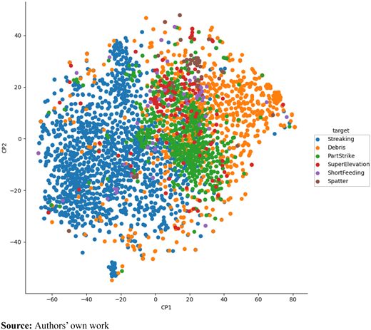
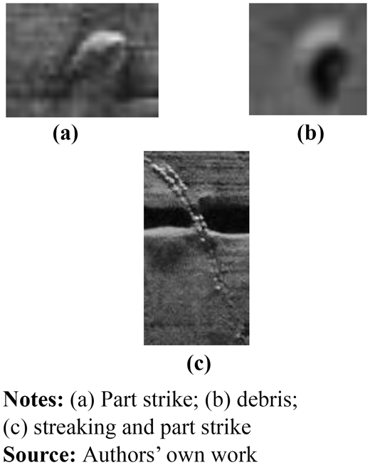
When evaluating the scatter plot in Figure 1, there appear to be three major clusters of data points, with a few smaller clusters scattered in between. The three main clusters consist of the streaking, debris and part strike defect classes. When referring to Table 2 in the previous section, these are the defect classes with the highest number of training images which translates to more clustered data points. It also becomes clear that these data clusters are still closely grouped which is not ideal as typically there should be a greater distance between the different clusters. This means misclassification between streaking and part strike is possible, as well as between debris and part strike. When reviewing some of the images of these classes of defects, it becomes clear why these defects are closely related to each other. From the illustration in Figure 2a and 2b, it is visible that a part strike may sometimes have a close resemblance to debris. From Figure 2c it also becomes clear that in some of the training images, the streaking defect was often caused by the part strike defect, which means there is often a bit of streaking in the training image of the part strike defect, explaining this close relationship.
When delving further into the T-SNE analysis, another relationship is also identified between part super elevation and part strike. When evaluating the literature behind this defect, it was identified that the part strike defect is directly caused by part superelevation. This means a part strike will always be caused by the superelevation defect, however, in extreme cases the superelevation will not always be visible before the part will elevate far enough immediately after the fusion process to cause a part strike (Kleszczynski et al., 2012).
3.2 Basic design ideology
For the design of a system that can detect and classify powder bed defects not dependent on NN or DL, conventional image processing techniques can be used to detect the defects and classify them by making use of supervised and unsupervised ML techniques such as k-nearest neighbours (KNN) or support vector machines (SVM). The basic design idea is to break up the proposed system into two primary functions, namely, the defect detection and defect classification stage. The reason for following this strategy is the methods used for detecting objects or features in an image differ from the classification of features in an image. To detect defects on the powder bed surface, it is only necessary to identify changes to the powder bed surface, whereas to classify defects it would be necessary to identify specific features from the image to identify the type of defect.
3.2.1 Defect detection
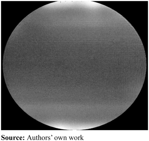
Under normal conditions, when a new layer of powder has been recoated or a layer of powder had been fused, the powder bed image will look typically like the image displayed in Figure 3. Although the colour of the powder bed might change depending on the type of material being used, the powder bed should ideally be smooth after the recoating operation.
For this study, the focus will only be on identifying powder bed defects in a metal AM machine manufacturing parts using stainless steel powders. However, from the literature, it was discovered that the training images for these types of materials work well with other types of metal powders or darker-coloured materials, except for light-coloured materials such as polymers which would possibly require different illumination methods to detect the defects on a lighter coloured surface (Scime and Beuth, 2018b).
Based upon the previously discussed studies, it was hypothesised that the method proposed by Scime and Beuth could be sped up since the entire surface of the powder bed was processed by the classification algorithm even if no defects were present. This process can take up a significant amount of time as ideally most of the captured layer images will not have any defects present on the powder bed surface. Therefore, it would make sense to make use of an algorithm that can detect changes on the powder bed surface and highlight the areas where changes were detected. If no changes were detected on the powder bed surface, the image is only stored for reference as no further processing or classification will be required.
One of the techniques that have been identified to compare an image for any possible changes when compared to a reference image is called structural similarity index metric (SSIM) (Wang et al., 2004). The SSIM is an image processing algorithm that can be used to determine the perceived quality of images. One of its other well-known applications is to use this functionality to determine the degree of similarity between two images. This is commonly used to determine if any changes have occurred in an image during the compression and decompression process (Wang et al., 2004). This function can be adapted to highlight the differences between two images as illustrated in Figure 4. It is used as an improved replacement for the more well-known methods such as mean squared error and peak signal-to-noise ratio (Wang et al., 2004).

For this study, the open-source implementation of SSIM will be used as implemented as part of the OpenCV image processing library. Since the SSIM function provides a mask image highlighting the areas where changes were detected between the two compared images, it is possible to do a contour detection on this masked image and the areas containing the changes can be “cut out” of the captured image and passed to an image classifier.
3.2.2 Defect classification
As discussed earlier in this article, one of the key features required by a powder bed defect classification system is the ability to distinguish between different classes of defects detected from the powder bed surface. While these classification abilities have been proven possible by studies performed by numerous authors, the most effective of these studies have involved using NN or DL algorithms (Scime and Beuth, 2018b; Westphal and Seitz, 2021; Du Rand et al., 2020).
Based upon the results achieved by Scime and Beuth (Scime and Beuth, 2018a), it was decided to re-visit the image patch classification strategy called bag-of-visual-words (BOVW). BOVW is a technique borrowed from the ML field of natural language processing called bag-of-words (BOW) used to extract features from a text to describe the occurrence of words in a given text (Zhang et al., 2010). In this sense, words are isolated from a given text to form a vocabulary, and a fixed-size vector is created for each of the words in the vocabulary. These vectors are combined to create a dictionary or “Bag of Words”. An ML model is then trained on this dictionary and can then identify these words from a given text and provide a result in which it calculated the total number of times each specific keyword was identified in a given text. Since it works like a normal dictionary, it does not retain any information regarding the order, structure or context of the words.
Since ML models can only work with numerical data, the BOW technique needs to convert all the features to a numerical vector, and, thus, the concept can be adapted to work with a variety of input data types, provided the necessary features can be isolated and the required vectors can be created (Gandhi, 2019).
When working with images, the process is like working with words. Images of the defects that are typically encountered are processed by a feature extraction system to extract specific features from the image, and these features are then used to create vectors which will form a “dictionary” of “visual” words. An ML model is then trained on these “visual words”. Once the ML model has been trained, an image can be processed using the same feature extraction system to extract specific features from the image, and these features are then used to create a new vector that will be compared to the existing BOVW to determine if there are any similarities to the defect vectors the ML model has been trained on. Based on the results supplied by the ML model, the image can be classified as belonging to a specific defect class.
To extract features from the training images to train the BOVW algorithm, an algorithm called scale invariant feature transform (SIFT) is used. A good feature extraction algorithm must be used for BOVW as the quality of the extracted feature has a direct impact on the accuracy of the image classification process (Wang et al., 2021). The SIFT algorithm is a method used to extract features from an image in the form of a set of key points and descriptors of the area around the key points. This information can then be used to detect similar patterns in other images (Lu et al., 2021). Since the original SIFT algorithm had been patented, there have been some improvements made to the algorithm, with the RootSIFT adaptation of the algorithm being used to great effect with BOVW (Mchlaughlin, 2020; Arandjelović and Zisserman, 2012). The RootSIFT feature extraction algorithm works in principle the same as the original SIFT algorithm, it just uses a Hellinger kernel to measure the similarity between descriptors instead of the Euclidean distance. This leads to a dramatic increase in performance with only minor coding changes required (Arandjelović and Zisserman, 2012).
One of the important features of BOW or BOVW is the algorithm can be applied to most types of classifier ML models. Based on the literature, the more commonly used ML models used are variants of decision trees, random forests and SVM (Qi et al., 2019; Aslan et al., 2020; Okafor et al., 2016). While some perform slightly better than others, most of these models are comparable in performance in terms of speed and accuracy. When working with unbalanced data sets, some models such as SVM perform better than others and can also prevent the model from overfitting with a bias to a specific class (Brownlee, 2020b).
3.3 Programming logic
Since the machine captures images of each layer of the part being manufactured and stores them in a folder on the control system machine, the algorithm will have to import the physical image file as soon as it is saved by the machine for further processing. As this proposed software algorithm will be running separately from the machine’s control system machine, a folder watchdog will be used by the algorithm to monitor the machine’s image storage folder. Once the watchdog detects that a new image has been created inside the folder, it will immediately load the image into memory for further processing by the algorithm. Before this function is initiated, an empty CSV file is created to be used by the algorithm to store the defect data. Alongside this, a benchmark image of a smoothly re-coated powder bed surface is imported, converted to greyscale and cropped for further use as part of the algorithm.
A breakdown of the process flow to be followed by the algorithm once an image has been stored is illustrated in Figure 5.
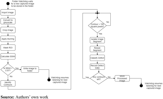
The highlights of the process followed by the algorithm are as follows: When the image is imported into the algorithm, the image is immediately converted from colour to greyscale, it is cropped to only show the powder bed surface, bilateral blurring is applied and the area surrounding the powder bed surface is masked out. It is important to note that the dimensions of the cropped image must match the dimensions of the cropped benchmark image.
Once the captured image has been pre-processed and masked, it is now ready for analysis by the main algorithms. Using the SSIM function as discussed in the previous section, the masked image is compared to the benchmark image to determine any differences between the two images. Once the difference has been determined, a binary image is created highlighting the areas of change between the images. This binary image is then processed by a contour detection function to determine the position of the detected differences After all the contours have been identified, the area of each contour is calculated, and contours having an area of larger than 150 square pixels will be processed further. This prevents the analysis of noise present in the image.
The identified contours are now to be processed by the classification portion of the algorithm. Each of the identified contours is then segmented from the originally masked image. The image segment is now resized without maintaining the aspect ratio to a fixed dimension of 100 pixels × 100 pixels. Since the original model was trained on images of a fixed dimension, these image segments must be resized to the same dimensions. After resizing, it is analysed using the RootSIFT feature extractor, and the image descriptors are then compared against the trained KNN model to calculate the feature vectors for the segment. These vectors are then analysed by the SVM ML model, and a prediction is made as to which defect class the segment belongs to. Since the segments are rectangular, the bounding box’s diagonal minimum and max coordinates are recorded as well as the image file name and the defect type and stored inside a CSV file for post-build analysis purposes. This defect classification process is repeated for each of the identified image contours until all the identified changes on the powder bed surface have been processed. The detected defect position and defect type are then drawn onto the originally captured image and a copy of this image is also stored for visual post-build verification purposes as shown in Figure 6.
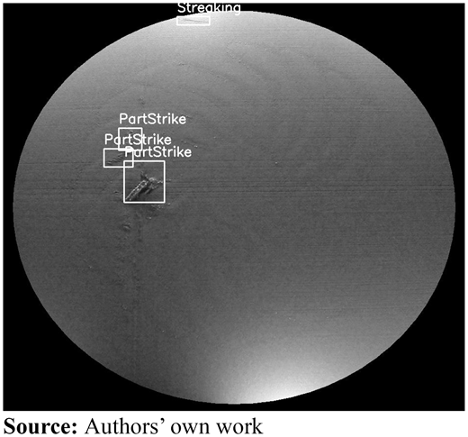
Once the image has been completely processed, the folder watchdog will resume watching the folder where the captured images awaiting the new captured layer image. This process will repeat until the operator stops the program at the end of the build job.
4. Experimental findings
4.1 Machine learning model training results
4.1.1 Machine learning model training parameters
Once all the training data was collected and processed, the training of the ML model could commence. To determine which combination of hyperparameters delivers the highest precision, recall and accuracy when training the ML model, it was necessary to test a variety of combinations to determine the optimal set of hyperparameters.
To enable this, a range of parameters is defined for the ML model, which for this study will be a Weighted SVM model. For this type of model, four hyperparameters can be adjusted to tune the performance of the model. To test all the different combinations of hyperparameters, a function called GridSearch is used to train the ML model. Once the optimal parameters have been determined, the model is trained with the best parameters selected from GridSearch. The range of tested hyperparameters is listed as follows:
Gamma: 0.01, 0.001, 0.0001;
1, 10, 100, 1,000;
Kernel: rbf, linear, poly and sigmoid; and
Class weight: balanced
Since the training data set was imbalanced, the decision was made to make use of the balanced set of class weights to try and prevent the model from overfitting on the defect classes that have more training images. While it is possible to specify custom weights for each of the defect classes, it is a more sensible choice to make use of the heuristic that forms part of the balanced class weights to automatically determine the optimal class weights (Brownlee, 2020b).
4.1.2 Machine learning model evaluation parameters
Once the training process has been concluded, it is important to evaluate the performance of the model using the test data set. This evaluation process is used to benchmark the performance of the model for each of the individual defect classes. Since there are a total of six defect classes, it is important that not only the global accuracy of the entire model is considered, but the precision and recall for each of the individual defect classes. This is because the overall precision and recall will not be an accurate reflection of the true capability of a multi-class trained model.
Before discussing the performance of the ML model, it is necessary to briefly discuss the parameters used to evaluate the model. These parameters include precision, recall, accuracy and a confusion matrix. Although several parameters can be used to evaluate the performance of an ML model, these four parameters are by far the most common. Before calculating any of these evaluation parameters, four terms must be defined when working with them. All the evaluation parameters are calculated using these terms, and, thus, need to be described to understand their background. These terms are true positive (TP), true negative (TN), FP and false negative (FN) (Dalianis, 2018).
TP: the model correctly predicts an image belonging to a specific class.
TN: the model correctly predicts an image not belonging to a specific given class.
FP: the model incorrectly predicts an image belonging to a specific class.
FN: the model incorrectly predicts that an image does not belong to a specific class.
The first parameter to be discussed is precision. This parameter is the ratio of TPs to the sum of all the positive predictions and can be calculated using the formula illustrated in equation (1):
The second parameter to be discussed is recall. This parameter is the ratio of TPs to the sum of all the actual positive cases (also called ground truth). Recall can be calculated using the formula illustrated in equation (2):
While precision and recall are valuable parameters used to evaluate the performance of an ML model, it is advisable not to use them in isolation. It is impossible to improve both precision and recall at the same time as they are inversely proportional to each other, one of these parameters must be selected as the primary parameter based on the application in which the ML model will be used (Afonja, 2017). For this study, the detected defect must be correctly classified, as the envisaged future work from this project will be to develop a closed-loop feedback system in which this defect classification will be used to feed the feedback loop. This means if a defect is incorrectly classified, inappropriate corrective actions might be taken which could have catastrophic consequences.
The third evaluation parameter to be evaluated is the accuracy parameter. As discussed earlier, using accuracy alone to evaluate an ML model is not ideal. A model may have high accuracy, but the precision may be low. In such a case the ML model may appear to have an impressive performance, but in reality, the predicted results may be spread out (Dalianis, 2018). Accuracy is still a useful parameter to get a global idea of the performance of a model. The formula used to calculate the accuracy of a given model is illustrated in equation (3):
The last technique used to evaluate the performance of an ML model is more of a visualisation technique as illustrated in Figure 7 than a parameter and is called a confusion matrix. Confusion matrix is primarily used to visualise the performance of a given model in terms of TP, TN, FP and FN.
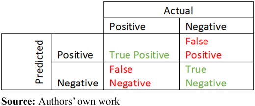
A confusion matrix can be used to determine the errors typically made by a model since the predicted values provided by the model are compared to the ground truth values (Beauxis-Aussalet and Hardman, 2014). This technique is particularly useful to identify if a model is consistently misclassifying a specific class or mixing up the predictions between classes. When evaluating an ML model trained on multiple classes, the confusion matrix can be expanded to accommodate each of the classes.
4.1.3 Machine learning model training results
Once the model completed the training process, the model was evaluated on the test data set, and the results were recorded for further analysis. Illustrated in Table 3 is the performance of the trained ML model once it has been evaluated on the test data set.
ML model evaluation performance
| Defect | Precision | Recall |
|---|---|---|
| Debris | 0.84 | 0.65 |
| Part strike | 0.70 | 0.68 |
| Short feeding | 0.10 | 0.30 |
| Streaking | 0.95 | 0.88 |
| Super elevation | 0.17 | 0.37 |
| Spatter | 0.24 | 0.77 |
| Macro avg | 0.5 | 0.61 |
| Weighted avg | 0.82 | 0.75 |
Source:
Upon evaluation of the performance of the ML model, some of the classes of defects appeared to perform well, whereas other defect classes did not perform well at all. Referring to the analysis of the training data set, the prediction was made that the model may have some difficulty in training and predicting these classes of defects as the amount of training data available for these classes was slim.
Lastly, it is necessary to evaluate the performance of the ML model using a confusion matrix. For this part of the evaluation, it is important to look at which defects the model had problems classifying, and which defects had the most misclassification problems. A graphical illustration of the confusion matrix is demonstrated in Figure 8.
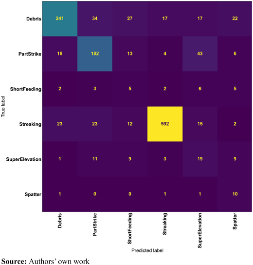
Confusion matrix for the trained model (the numbers in each cell of the matrix indicates the number of images classified for that specific class of defect)
Confusion matrix for the trained model (the numbers in each cell of the matrix indicates the number of images classified for that specific class of defect)
When looking at the confusion matrix displayed in Figure 8, some interesting observations can be made. The first striking detail is there are only three classes of defects predicted where the majority of the defect images where correctly classified. When comparing this observation to the data illustrated in Table 3, the classes of defects with the highest precision and recall values also had the highest number of correctly predicted defect classes. Thus, the ML model was trained to a high level of confidence for those defects. When referring to sub-section 3.2 about the data analysis, the hypothesis was confirmed about the defect classes having the highest number of training images achieving the highest levels of precision and recall.
When examining the other defect classes, some of them suffered from severe misclassification. The one with the highest level of this misclassification is superelevation. This defect was misclassified as part strike more often than it was correctly classified. This misclassification is supported by literature since a part strike is caused by a superelevation of a part, and, thus, it would make sense that it could easily be misclassified as a part strike.
4.2 The case study build detail
Once the ML model has been evaluated, it is necessary to test the algorithm under production conditions. For this case study, a build was monitored of a set of parts manufactured out of stainless-steel metal powder. The build took 13 h and 26 min to complete. Although the build did finish all the layers, several defects occurred during the process having the potential to cause severe damage to the build. A breakdown of the build is provided in Table 4.
4.3 Post-build data analysis
With the build completed, the defect classification data was extracted from the machine for detailed analysis. This post-build analysis is not only valuable to determine the efficacy of the defect classification algorithm but also in determining what problems may have occurred during the build.
The first step was to process the CSV file containing the defect data and to determine the number of defects recorded by the algorithm. Although there may be cases where defects may have been incorrectly classified, it is important to evaluate the total number of defect classifications made by the algorithm. From this point, each of the captured images with the highlighted defects was analysed by a human operator to determine whether any defects were not detected at all, and if there were any incorrectly classified. These statistics can then be used to determine the real-world accuracy of the BOVW algorithms in classifying the defects according to type.
From the data, the following defect breakdown could be made as shown in Table 5, highlighting all the defects the algorithm had recorded during the image analysis.
Case study defect analysis
| Defect type | Precision | Recall | Accuracy |
|---|---|---|---|
| Debris | 0.55 | 0.72 | 0.18 |
| Streaking | 0.94 | 0.99 | 0.93 |
| Short feeding | 0.56 | 0.50 | 0.20 |
| Part strike | 0.92 | 0.99 | 0.98 |
Source:
When evaluating the data recorded from the case study build, two of the defect classes performed well and had a precision, recall and accuracy of above 0.9. The remainder of the classes performed much poorer. While conducting the visual validation of the defects, some interesting observations were made. When looking at the incorrectly classified defects, it was seen that the streaking defect was misclassified as the debris defect several times. This was a strange phenomenon as the debris defect had a high precision and recall value during the model evaluation. Upon closer observation, it was discovered that because all the images must be resized without maintaining the aspect ratio before they can be passed to the feature extractor, it often happened after the image patch was resized, that the streaking and debris defects looked similar. This means this resizing strategy may need to be re-evaluated to prevent the feature extractor from becoming confused between the two defect classes. While there was not a lot of debris present during the build, many of the defects classified as debris were incorrect.
Several debris defects were not detected by the algorithm at all. When re-evaluating these images using the SSIM algorithm, it was seen these defects were often considered noise due to their small size and thus were never passed to the ML model for classification.
Another problematic defect for the ML model was the short feeding defect. Unfortunately, when looking at the evaluation data for the ML model, this was expected as the model had a low precision and recall for this class of defect. When referring to the training data set breakdown in the previous section, it was seen that this defect class only had a small number of training images, which means the model could not be trained to a level where it could reliably predict (> 0.5%) a defect as belonging to the short feeding class.
Lastly, the two defect classes that performed well were the streaking and part strike defects. This was expected as these defect classes had high recall and precision values. When examining the training data set, it could be noted that these defect classes had the highest number of training images, which means the ML model had a larger number of features to learn from. Although some defects were incorrectly classified as streaking, this was a small percentage. Most of these misclassifications were due to defects containing a small piece of streaking, but some of the detected defects were completely misclassified.
4.4 Machine learning model conclusions
As discussed in the introduction, several studies in the literature have focused on making use of a variety of ML and DL models to detect and classify powder bed surface defects from captured layer images. The downside of using DL technologies is that they require a significant number of computational resources. Although these technologies provide impressive performance in terms of classification accuracy and detection speed, this performance is computationally costly. For this reason, this study focused on the use of traditional ML models for defect classification.
A final factor to consider when evaluating models is the hypothesis made of speeding up the defect detection and classification process. While a balanced level of defect classification accuracy could not be maintained for all the discussed defect classes, it was demonstrated that the defects with a high number of training images could be accurately detected. Analysing the performance of the defect detection and classification Algorithm a surprising discovery was made. Many studies focusing on the detection and classification of defects from powder bed images do not disclose their image processing times, one study conducted by Scime and Beuth did disclose that their designed algorithm could detect and classify defects in 7 s when using the BOVW technique and could more accurately do so in 4 s when using a NN (Scime and Beuth, 2018b). While it would be ideal to compare this BOVW to a NN trained on the same training data set, the purpose of this study was to benchmark the BOVW techniques in detecting powder bed defects to existing literature to see how this technique can be improved.
While evaluating the case study build, the time taken by the algorithm to analyse the image was recorded and the breakdown of the times is shown in Table 6. It can be noted that the times varied depending on the number of defects present in the image.
Image processing times
| Average time | 202 ms |
| Minimum time | 144 ms |
| Maximum time | 606 ms |
Source:
Looking at the breakdown of the recorded times achieved by the algorithm, a big increase in processing time was achieved compared to what was reported in the literature. The most important factor is that this performance was achieved by only making use of a CPU, which eliminated the need for a high-end GPU to enable processing the images at a higher speed than would be required for a YOLO model. One factor that increased the speed of the proposed algorithm is that only the areas of the image that had detected changes were analysed by the ML model, thus, reducing the number of image patches to be analysed.
While future work is required to enable increased accuracy of all the defect classes, this study did manage to achieve its objective of developing a defect detection and classification algorithm that can process powder bed images at a high speed with an acceptable level of accuracy for a prototype system.
5. Conclusions and future work
In conclusion, this study focused on the practical use of more traditional image processing techniques and ML models to develop an algorithm to both detect and classify powder bed surface defects from surface images. The study focused on current methods used by other researchers in the literature and identified some of the shortcomings these methods had concerning their high computational resource burden. Based on literature and current technologies available on the market, a method was proposed in which standard image processing techniques could be used to detect defects from the powder bed surface images, and a more traditional ML model such as a SVM could be used to classify the defects according to type. These techniques were combined to create a BOVW algorithm as used in similar applications, howbeit with less-than-optimal image processing speed.
The ML model was trained on a defect training data set, and the entire algorithm was used to process a real-world build job under real-world conditions. The data recorded from this build was then used to evaluate how well the entire algorithm along with the ML model performed. From the data recorded, it was seen that the proposed algorithm could process an image in an average time of 202 ms, whereas from literature, the average time taken to process an image was between 4 s for a NN to 7 s using BOVW (Scime and Beuth, 2018b). This showed that conventional techniques still have a significant performance advantage when compared to newer methods as conventional techniques can still process images at a high speed without requiring specialised hardware or GPUs. On the accuracy front, it was seen that some of the defect classes did have an accuracy of over 80%, whereas other defect classes had a low accuracy of less than 10%. The reason for this low accuracy could be attributed to the lack of a sufficient number of training images for these specific defect classes. The defects that had a healthy number of training images did achieve a high level of accuracy.
Based upon these discoveries, it can be concluded that even with the recent advances made in the field of DL, there still exists a place for the traditional image processing techniques and ML models to be used in production environments such as the field of AM.
For future work, it will be necessary to increase the amount of training images, so that all the classes are more evenly balanced in terms of training data. Based on the outcome of the experiments conducted during this study, this would be one of the best solutions to increase the precision and recall of the ML model, and, thus, increase the accuracy of the overall system.
The research was funded by the Collaborative Programme in Additive Manufacturing. Grant MoA No: CSIR-NLC-CPAM-21-MOA-VUT-01.

