


In this study, response surface methodology (RSM) is applied to a three-point bending stiffness analysis of low-cost material (PLA) specimens printed using FDM technology to analyze the performance of different internal lattice structures (Octet and IsoTruss principally). The purpose of this study is to extend the definition from a discrete (lattice) model to an analytical one for its use in subsequent design phases, capable of optimizing the type of cell to be used and its defining parameters to find the best stiffness-to-weight ratio.
The representative function of their mechanical behavior is extrapolated through a two-variable polynomial model based on the cell size and the thickness of the beam elements characterizing it. The polynomial is obtained thanks to several tests performed according to the scheme of RSM. An analysis on the estimation errors due to discontinuities in the physical specimens is also conducted. Physical tests applied to the specimens showed some divergences from the virtual (ideal) behavior of the specimens.
The study allowed to validate the RSM models proposed to predict the behavior of the system as the size, thickness and type of cells vary. Changes in stiffness and weight of specimens follow linear and quadratic models, respectively. This generally allows to find optimal design points where the stiffness-to-weight ratio is at its highest.
Although the literature provides numerous references to studies characterizing and parameterizing lattice structures, the industrial/practical applications concerning lattice structures are often still detached from theoretical research and limited to achieving functioning models rather than optimal ones. The approach here described is also aimed at overcoming this limitation. The software used for the design is nTop. Subsequent three-point bending tests have validated the reliability of the model derived from the method’s application.
1. Introduction
Lattice structures represent a pivotal facet in contemporary engineering design (Bacciaglia et al., 2022). These are characterized by repetitive patterns of one or more geometrical cells distributed inside the volume or onto the surfaces of a mechanical part. The “'classic” porous structures are composed of patterns of beams with a defined thickness distributed within a cell (typically cubic) according to a specific arrangement. Among the most recognized and industrially employed types are Cubic (as body centered or face centered) (Ma et al., 2023), Diamond, Fluorite, Octet (Korshunova et al., 2021; Nam et al., 2023), Weaire-Phelan, IsoTruss, Kelvin cell (Wang et al., 2023a), to name a few. They are generally easy to print and excellent for significantly reducing the weight of the mechanical component, thereby lowering its relative density (Song et al., 2021). These cells are actual lattice structures consisting of small beams (Latture et al., 2018) arranged in space according to directions and angles characterizing each of them. These geometries generally cause a specific cell to deform/offer resistance along preferential directions. Other cell types, such as triply periodic minimal surfaces (TPMS) (Zhang et al., 2024; Günther et al., 2023), exhibit a spatial form characterized by well-known mathematical equations. These cells typically offer high stiffness and greater energy absorption capacities in case of impacts compared to beam-based cells, but they are more challenging to manufacture through printing processes (Echeta et al., 2020; Cai et al., 2022). However, 3D printing often influences the quality of the print by leading to defects such as non-filling, material shrinkage, localized deformations (Ferretti et al., 2023; Liverani et al., 2023; Ciccone et al., 2023). Perhaps the most well-known and used lattice type for manufacturing is the Gyroid structure, followed by others such as the Diamond, SplitP, Lidinoid, Schwarz (Cai et al., 2022), Neovius. A comprehensive representation of the most used cells in the field of scientific research/3D prototyping is provided in Figure 1.
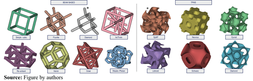
Possible types of infill cells: beam-based classic cells and triply periodic minimal surfaces
Possible types of infill cells: beam-based classic cells and triply periodic minimal surfaces
In direct comparison to conventional foams and honeycombs, lattice structures emerge as superior counterparts, particularly in terms of mechanical prowess (Dong et al., 2017; Uddin et al., 2024; McDonnell et al., 2024). The overarching objective, as addressed in numerous scientific publications on the subject, is generally directed toward defining stiffness models (Daynes, 2023; Wang et al., 2023b; Stallard et al., 2023) for various cell types based on the differing magnitudes of loads and constraints they encounter. These studies encompass the assessment of the mechanical response (Imediegwu et al., 2023) of polymeric lattice structures (Eren et al., 2022), structural analysis of sandwich beams with lattice core (Ghannadpour et al., 2022), stiffness optimization in sandwich structures with isotropic lattice core (Zhu et al., 2024), experimental and analytical investigation of bioinspired lattice structures (Doodi and Balamurali, 2023), production and mechanical properties analysis of steel strut-based lattice structures (Caiazzo et al., 2022) and the mechanical behavior of a novel lattice configuration (Ma et al., 2024). Similar case studies exist but are focused on the analysis of energy absorption (Niutta et al., 2022; Boursier Niutta et al., 2022; Khan et al., 2024). Notable contributions include the crashworthiness design of functional gradient bionic structures under axial impact loading by Wang et al. (Wang et al., 2023c), the exploration of bending crashworthiness in smooth-shell lattice-filled structures by Yin et al. (2022) and a study on the design and impact energy absorption of Voronoi porous structures with tunable Poisson’s ratio by Zou et al. (2024). Li et al. (2021) delve into the characterization of energy absorption for side hierarchical structures under axial and oblique loading conditions, while Alkhatib et al. (2023) focus on the isotropic energy absorption of topology-optimized lattice structures. Other studies concern sound applications with customizable lattice cells (Li et al., 2023).
Often, there is a significant use of design of experiments (DOE) and/or response surface methodology (RSM) based on analysis of variance (ANOVA) in these research studies, as known in literature (Mushtaq et al., 2022; Ali et al., 2023; Li et al., 2018; Mushtaq et al., 2023; Vălean et al., 2020; Bacciaglia et al., 2021). This is usually due to the difficulty in defining a mathematical model representative of these structures, given their complex shapes and the general nonlinearity of their mechanical behavior. This integration is usually applied to the design of lattice structures aimed at identifying optimal parameters for cell design and printing, with the goal of minimizing technical defects. Aslani et al. (2020) present a quality performance evaluation of thin-walled PLA 3D printed parts using the Taguchi Method and Grey Relational Analysis, shedding light on the robustness of 3D printing techniques in lattice structure fabrication. Vaissier et al. (2019) contribute to the understanding of thermal dissipation through their parametric design of graded truss lattice structures (Latture et al., 2018), demonstrating the potential for enhanced thermal management. Meanwhile, Di Prima et al. (2024) investigate the influence of build parameters on strut thickness and mechanical performance in additively manufactured titanium lattice structures, elucidating critical factors in the production process. An additional step forward in this field has been taken thanks to artificial intelligence (AI) often integrated also with DOE/RSM studies. Eren et al. (2024) present a deep learning-enabled design for tailored mechanical properties of selective laser melting-manufactured metallic lattice structures. Challapalli et al. (2021) propose an inverse machine learning framework for optimizing lightweight metamaterials, showcasing the potential of AI in metamaterial design. Yüksel et al. (2023) provide a comprehensive review of AI applications in engineering design, offering a broader perspective on the transformative role of AI. Siegkas (2022) explores the generation of 3D porous structures using machine learning and additive manufacturing, highlighting the synergy between AI and manufacturing processes. Additionally, Yüksel et al. (2024) investigate the mechanical properties of additively manufactured lattice structures designed through deep learning, emphasizing the role of AI in tailoring material behavior. Nasiri and Khosravani (Nasiri and Khosravani, 2021) delve into machine learning’s predictive capabilities for the mechanical behavior of additively manufactured parts, and Hassanin et al. (2020) explore the control of properties in additively manufactured cellular structures using machine learning approaches. These works collectively underscore the transformative impact of AI in redefining the boundaries of lattice structure design and optimization. However, the main limitation associated with the integration of AI is related to the large amount of data required to train neural networks. Prototyping times linked to 3D printing of complex geometries, coupled with test realization times, can often prove to be excessive. Frequently, the use of established methodologies such as DOE, constructed on the minimum number of trials necessary for the study of the system, remains favorable, as evidenced in the following study.
Although the literature provides numerous references to types, data and properties of lattice structures (Maconachie et al., 2019; Chen et al., 2023; Pan et al., 2020), their practical application still proves challenging. The choice of the cell type to employ frequently depends on the shape of the component being designed and the loads to which it is subjected. For instance, cubic cells perform well under tension but poorly under bending or compression (primarily due to local buckling phenomena). Even in the hypothetical scenario where the optimal cell type is known with certainty, understanding the optimal values for cell dimensions, including its thickness (beam diameter in the case of classic cells/surface thickness in the case of TPMS), remains a complex task.
For these reasons, the following study proposes an approach aimed at obtaining a highly reliable mathematical model (in the form of an n-variable polynomial) to assess the variation in structural stiffness as the main representative parameters of the model change. These parameters include the size, beam thickness and type of cell used. The reliability of the derived RSM model is verified by comparing its results with those obtained from every single FEM calculation applying various cell dimensions and thicknesses of the constituent beam elements. Following this application, an analysis of the local error obtained from the application of the RSM methodology concerning the variation of cell size is conducted. This variable is continuous and therefore suitable for the RSM methodology. However, the presence of some undesired effects in the 3D printing process is one of the main causes of the overall imprecision observed in the model, as described later. The specimens used in the study are also tested in three-point bending tests necessary to validate their virtual models and derive the real structural stiffness. The specimens are printed with PLA using FDM technology, in accordance with relevant standards and project requirements, as described later.
2. Materials and methods
The first phase of the study is designed to immediately derive the most rigid structural models for the three-point bending geometry considered in the following RSM analysis. This avoids excessively increasing the number of combined tests on the PLA physical specimens. To achieve this, several specimens of the same geometric dimensions are considered. The specimens are in line with ASTM D7249 standards, although slightly resized. The reason for this resizing is related to the maximum printing volume of the Artillery Sidewinder X1 (300 × 300 × 400 mm) printer used for subsequent 3D prototyping. Other cases in the literature implement resizing when the specimen’s size is not particularly relevant for the study’s tests (Austermann et al., 2019) or variance analysis. The specimens are rectangular prisms made entirely of PLA, a low-cost polymer material that is easy to print. The dimension of the internal core is 180 x 36 x 18 mm. This is the volume that changes in each test based on the type of cell and its dimensions. Two continuous layers of PLA, each 1 mm thick, are applied to the upper and lower faces. The full specimen size is then 180 x 36 x 20 mm. The main reason for this choice is to minimize the possibility of local crushing effects at the three contact points of the bending test excessively influencing the overall deformation of the specimen. This deformation serves to evaluate the representative stiffness of each specimen, assessed each time as the ratio between the applied load and the vertical displacement in the midpoint recorded at the bottom of the specimen. In fact, both in virtual and experimental tests, the effect of compression due to the punch at the midpoint usually resulted in slightly greater vertical displacements on the upper face of the specimen compared to the lower one. A schematization of the test set up and a representation of this effect is proposed in Figure 2.
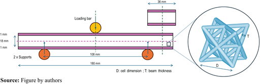
Schematization of three-point bending test and specimen dimensions according to ASTM D7249
Schematization of three-point bending test and specimen dimensions according to ASTM D7249
Another reason for choosing these specific values is related to the need of multiple sizes nested within each other. The idea was to analyze large dimensional variations of the cells and their thicknesses, as subsequently specified, specifically using only full lattice cells (this means that their sizes were necessarily submultiple of the core volume dimensions). In fact, if the three dimensions (length, height, depth) of the specimen are not all multiples of the length of the sides of the cubic cells, these will remain partly incomplete in certain areas of the internal core. In general, this happens in the interface areas with the upper and lower faces of the specimen. In an RSM analysis, the system analyzed should remain the same even if it foresees a continuous variation of its parameters. The approach is indeed valid if specimens always have complete cells although their dimensions are changing at each simulation. This is an efficient way to get a correct final regression equations in authors’ opinion. Using cells with 3 or 9 mm sides (variable D), it is then convenient from this point of view. The core dimensions (18, 36 and 180 mm) are in fact multiples of each. In addition, their mean value (6 mm) is also a divisor of these values (this is useful in the RSM model described later). Defining the range in which to vary the size of the cells is the first step. The choice of the most useful specimen sizes follows accordingly. More details on this are described below.
Each virtual test should be validated with experimental analyses performed on real specimens. In this case, the high number of design parameters increases the time of experimentation. For this reason, it was necessary to look for the types of cells offering the best stiffness in subsequent bending tests. The first stiffness analysis was conducted maintaining a cell size of 6 mm and allowing thickness variations for this reason. To already identify the stiffness trends in this analysis (non-RSM), four thickness values (variable T) were chosen as inputs. These were: 1 mm, 1.5 mm, 2 mm, 2.5 mm. Here, the use of beam elements is employed in FEM simulations to expedite processing and computation times. The beam finite element is ideal for use in the analysis of lattice structures (not for TPMS ones, only for trabecular ones). Its simplest version (2 nodes) allows displacements at the ends in the three Cartesian directions to model the application of all possible external loads (tensile/compression, shear, bending moment). In addition, the beam element of nTop (the software used for the design and virtual simulation phases) also admits the version with three or four nodes (one or two internal, respectively). However, it is not possible to evaluate the local stress increase due to carving effects in the model using it. This can be considered as one of its general limitations.
To clarify these last concepts, an image referencing some of the issues described in the model analysis is provided in Figure 3.
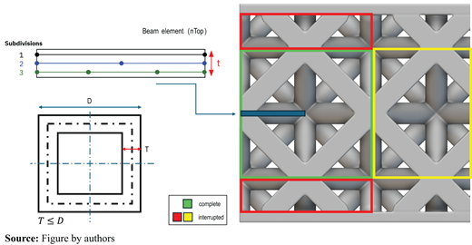
Beam element for FEM analysis and representation of interrupted octet cells within the lattice of a sample specimen
Beam element for FEM analysis and representation of interrupted octet cells within the lattice of a sample specimen
Another consideration concerns the typical anisotropy that 3D printed specimens exhibit in characterization tests. This issue is well-documented in the literature (Ali et al., 2023; Li et al., 2018; Mushtaq et al., 2023; Vălean et al., 2020) and during the prototyping phases, it is usually necessary to consider the principal printing direction (for example, the one in which the actual Young’s modulus offered by the specimens is greater). The material considered in the following tests is PLA (4 GPa as Young’s modulus and 0.35 as Poisson’s ratio used in virtual simulations). Using small-sized print layers (max 0.1 mm) in printing helps attenuate the specimens’ anisotropic behavior (Bacciaglia and Ceruti, 2023). All specimens were printed horizontally to ensure the best resistance capability along the horizontal direction of tensile/compressive fibers due to bending. Furthermore, print orientation constitutes a variable that would potentially need to be added to the system because it alters the mechanical behavior of the material. As can be inferred, these and further considerations regarding 3D prototyping do not pertain to the virtual analysis of the models. This approximation was considered valid because neither the virtual nor experimental tests focused on fracture tests. The tests conducted on the specimens were solely related to stiffness analysis in the discussed study (evaluated for small displacements).
Once the specimens with the best stiffness were identified, the RSM analysis followed. The dimensional range of the edge of the cubic cells was defined from 3 mm to 9 mm and represented with letter D. The average value between the two is easy to calculate and equals 6 mm. As can be seen, the ratio between the size of the sides of the core and these values always leads to integer values, guaranteeing in each analyzed combination an exact internal distribution of cells (cells cut in half or, in general, incomplete is avoided). The RSM model is of the face-centered type (alpha = 1). This is the best choice to avoid tests with cell sizes that are not divisible by those of the core, as previously underlined. If ANOVA leads to a predominantly linear or quadratic two-variable model, the characteristic regression equations will be of the first or second order, respectively, as shown in Figure 4.
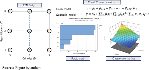
RSM analysis diagram with examples of linear or quadratic regression polynomials, Pareto diagram and 3D plots of a sample output
RSM analysis diagram with examples of linear or quadratic regression polynomials, Pareto diagram and 3D plots of a sample output
The final RSM model had to predict the maximum vertical displacement along the z-axis of the model. In general, there is no full linearity in the output, as shown in the results section. The range of variability of the thicknesses of the beams (their diameters) goes from 1 mm to 3 mm. This variable is represented with letter T in the manuscript. The value of 1 mm is large enough to guarantee that at least 10 layers of 0.1 mm cover it, while 3 mm (maximum) maintain a sufficiently wide range of manufacturable specimens. In fact, it is an adequate value for cells from 3 mm to 9 mm. The ASTM D7249 standard also provides guidelines for the optimal setup of the specimen test. As stated in Figure 2, the distance between the two supports is proportional to the length of the specimen and should not be chosen randomly. The load should be applied at the exact midpoint of the specimen. In the virtual and experimental tests described below, a load of 2000 N was used for the three-point bending test (the value may be high for tests on real specimens, as specified below, as it leads to the exceeding of the elastic response range of the specimens but has no relevance on purely virtual linear elastic tests).
Once the virtual RSM tests have been performed on the cells selected from the first stiffness analysis, it is possible to analyze which variables have the greatest effect on the system. An RSM analysis allows the evaluation of nonlinear pro-proportionality (as in classical factorial DOE) up to the sixth order. This is possible without much effort thanks to the help of applications such as Design Expert or Minitab (the latter, however, is limited to the second order). ANOVA useful for calculating the sums of squares of the different variables allow to weigh their effect on the results. Associated p-value analyses allow to immediately identify which ones are impactful and which have little effect on results. If a variable does not have a sufficiently low p-value (close to 0), it can be excluded from the polynomial regression analysis. The tests required a 95% reliability on the model here, which is why the p-values sought had to be less than 0.05. For the different types of cells analyzed with the RSM methodology, an n-order regression equation was then obtained (the second-order one, i.e. quadratic, resulted always optimal as shown in result section). This was necessary to link the variability of cell thicknesses and sides to the displacement (and stiffness) outputs. The overlapping graphic plots of the two outputs considered in these models allow to evaluate any n-tuples (cell side, beam thickness, cell type) of the analysis domain in which a small percentage reduction in stiffness is obtained compared to the solid material specimen in the face of a large lightening. This already offers a considerable technical starting point for the design. The classic contour plots then make it possible to highlight any optimal design points if they fall within the domain considered. Otherwise, an analysis of the gradients (growth rates) of the output functions in the same graphs is already sufficient to identify where the optimum points might be found.
A final comparison between some of the results predicted by the RSM model and the actual results of virtual (and experimental) tests is useful to identify the points where it is most divergent. Any macro-forecast errors (even if few and localized) could be due to the great variability in the mechanical behavior of the specimens. The internal porosity of the material makes its prediction more difficult, often far from the classic analytical model of the elastic line that can be used here as a first approximation. It estimates the inflected deformation of the specimen and is based on the following starting differential equation (1):
In it, M(x) is the value of bending moment along the length, E is the Young’s modulus of the beam and I is its surface moment of inertia (both constants on the x-domain). The x domain starts from one of the supports and it is directed toward the other one. The parts of the beam specimen outside these supports are not considered in this equation (in fact, they are not stressed). Non-constant is the value of the bending moment due to the applied load F (Figure 2), zero at the hinged ends and maximum at the centerline and equal to the product of the load F and half the length of the beam. Solving the differential equation results in equation (2):
The terms c1 and c2 emerge from the integration process and need to be analyzed for the specific case at hand. Knowing that w(x = 0) = 0 and w′(x = l/2) = 0 since it is the point of maximum deflection and at this point the tangent to the beam’s curvature is horizontal, the two values can be easily obtained by substitution, as follows in equation (3):
At the centerline point (x = l/2) it is in fact equal to the well-known Euler-Bernoulli equation (4):
3. Results
The first series of virtual analyses on the specimens allow to map the trend of the stiffness values in relation to the thickness variability alone. An analysis of this type precedes the RSM analysis but is useful for having a simple reference for comparison with subsequent multivariable analyses. In fact, if the graphical solution of a two-variable RSM approach is a continuous multidimensional curve in space (a plane in the case of linearity, paraboloids in the case of second-order relations and so on), intersecting it with a shear plane whose points are the pairs (D;T) in which the cell size is kept constant should yield similar patterns on the thickness domain.
The cubic cells analyzed were initially of ten different types: Simple cubic, Body centered, Face centered, IsoTruss, Diamond, Fluorite, Kelvin, Octet, Weaire-Phelan, Reentrant. The design of the specimens and the virtual simulation test was done with nTop, setting the dimensions of the standard specimen (20x36x180 mm), a load of 1000 N on the centerline and two lateral supports typical of three-point bending as in Figure 2. The thickness variability was 1, 1.5, 2, 2.5 mm. The load is applied over an area of 12x36 mm on the upper face to better represent the future experimental test. The real importance of the results, however, lies in their variation rather than in their values. Two cells (Simple cubic and Reentrant) were immediately found to be highly yielding and unsuitable for the following stiffness analyses, as shown in Figure 5. The table shows the values of vertical displacement (in mm) recorded in the transverse centerline on the upper face of the specimen and on the lower one, for the reasons explained in the previous section (Material and Methods). Except for the two clearly worse cells, we proceeded with the creation of the graph shown in Figure 5. As can be seen, the relationship between the increase in the thicknesses and the displacements recorded does not follow a linear model. Second- and third-order polynomial models, in general, apply well to these distributions with very high average R2 coefficients, close to 0.98 (simply verifiable), as described later.
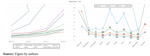
Displacement (z-axis) measured by FEM analysis on specimens of different cell types and thicknesses to highlight the most rigid specimens for three-point bending
Displacement (z-axis) measured by FEM analysis on specimens of different cell types and thicknesses to highlight the most rigid specimens for three-point bending
The graph helps to understand which models are best for the geometry, loads and constraints considered. The Weare-Phelain cell lends itself well to this type of test, followed by the Octet and the IsoTruss. For thicknesses of 2.5 mm, minimum expected displacement values are on the order of 0.25 / 0.5 mm. They increase up to 1 mm in the case of thicknesses of 1.5 mm. Cells with simple cubic cells or reentrants show peaks that are too high and are not suitable to withstand this type of load. In order not to excessively increase the number of experimental tests, it is advisable to focus only on the study of the best two or three cells. After all, no further analyses (virtual or experimental) on specimens made with Weaire-Phelan cells have been considered to speed up and facilitate the printing process, preferring the Octet and the IsoTruss types (easier to 3D print). The results obtained for the other two cell types should be representative of all specimens’ general behavior.
The first RSM model was applied to structures of the Octet type. Two continuous factors (cubic cell size D and beam thickness T) were defined for the model in the ranges [3; 9] and [1; 3] mm respectively. Each trial was performed and evaluated according to the two-level factorial central composite design (α = 1) model. The model includes 4 cube points, 4 axial points and 5 center points in cubes. The total number of trials is 13 and the various results are summarized in Figure 6.
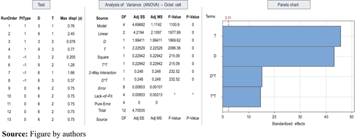
Scheme of tests, analysis of variance (ANOVA) and of the most influential variables for Octet cells in Pareto chart
Scheme of tests, analysis of variance (ANOVA) and of the most influential variables for Octet cells in Pareto chart
Similarly, the procedure was repeated with the same inputs for the IsoTruss specimens. The results obtained from these tests are roughly like those in Figure 6. The ANOVA table is not given for this reason so as not to weigh down the manuscript. Centerline displacement data will follow in the next figure. Once the analysis has been carried out, the two-variable regression function (D; T) that can better approximate them is easily obtained thanks to applications such as Minitab or Design Expert. As already stated, the order of this polynomial depends on the generic regression model that offers the best fitting value. The Octet linear model offered adjusted R2 and predicted R2 of 0.8547 and 0.7051, respectively. The quadratic equation had better values (0.9966 and 0.9810). The cubic model is “aliased.” This indicates that some interactions between the independent variables cannot be distinguished from other effects in the model. This is often the result of a limited number of experimental points compared to the number of terms. Similarly, the values of the adjusted R2 and predicted R2 of the IsoTruss model were 0.9864 and 0.9202. For these reasons, the quadratic model was the most suitable for its representation. The regression equations for the Octet and IsoTruss cells are as follows, respectively:
The effect of thickness is in both cases principally second order, while cells affect flexural stiffness linearly. Note that the term D2 does not appear in the equations because it was irrelevant from the ANOVA and the calculations of the p-values of the variables, as can be seen in Figure 6. Subsequently, the results extrapolated from the regression model were compared with those obtained from each individual simulation. This is useful in the case of real tests. These tests require time to prototype the specimens, to set up the machine for three-point bending and to carry them out. Simulations did not require particularly long times for setup and calculation (performed with nTop 4.17.3 on an Antec computer with a 2.5 GHz CPU, NVIDIA Quadro M5000 graphics card and 63.7 GB of RAM) also thanks to the use of beam FEM elements, the prototyping phases discussed later greatly lengthened the research time. This comparison is in general necessary to understand how close the regression model is to the individual case under consideration each time. As can be seen in Figure 7, in several cases the evaluation errors of the model reach peaks of up to 0.1 mm. In the procedure of comparison between the RSM data and those of the individual simulations, it was realized that the introduction of some higher-order terms allowed a better approximation between the two series. For this reason, new uncoded equations (i.e. referring to the integer terms D and T and not normalized to values from 0 to 1) have been derived to study the behavior of the model. References to the coefficients of these equations are in Figure 7.
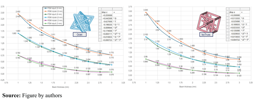
Comparison between vertical displacements derived from FEM analyses and RSM model predictions as cell thicknesses and sizes vary
Comparison between vertical displacements derived from FEM analyses and RSM model predictions as cell thicknesses and sizes vary
The main area of divergence is for the larger cells (9 mm). In a special case (D = 9 mm; T = 1.5 mm) the error is almost 0.2 mm. The reason is most likely related to the greater discontinuity of the model, characterized by greater displacements of the mesh elements and high local displacements along the centerline. Only small discrepancies emerge for the 3 and 6 mm cells, areas of analysis where the RSM surface works optimally. In all cases, for high values of thickness, the variation in stiffness tends to assume trends that can be well approximated with linear models. This is not true for small thicknesses. In general, a quadratic model is suitable for representing the stiffness behavior of these systems. However, it is only by adding higher-order terms that it is possible to approach the true behavior of the specimens with excellent accuracy. After the following series of analyses a further interesting result concerning the best combinations between stiffness and weight of the specimens is obtained. In fact, it has been noted that for Octet or IsoTruss cells of different sizes there is an optimal design point where the stiffness-to-weight ratio is maximum. To obtain this result, it was sufficient to calculate the percentage of material mass saved thanks to the use of lattice structures using the special nTop “weight savings” tool. The numerical results of this analysis are shown in the graph in Figure 8.
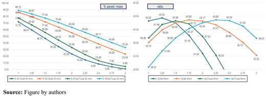
Plot of the percentage of mass saved as the thicknesses and dimensions of the cells vary and their relationship with the maximum displacements
Plot of the percentage of mass saved as the thicknesses and dimensions of the cells vary and their relationship with the maximum displacements
The percentage of saved mass is calculated every time by comparing the weight of each porous core to the fully filled core inside every specimen (relative density). This ratio is subtracted from the value 1 and then translated into a percentage. This means that the percentage of mass saved in the first of the two graphs should be intended as unprinted mass. As can be seen from the graphs, the variation in mass and stiffness does not always follow a direct proportionality and it is possible to identify an optimal weight/stiffness ratio in many cases. The change in mass, for example, follows almost linear models with respect to the change in displacement (and therefore in structural stiffness). The optimum points also fall in an area of the analysis domain where the thicknesses are quite small compared to the size of the cell and, therefore, physically plausible and manufacturable. In the case where D = 9 mm and T = 1.75 mm, Octet cells offer the best compromise. In the case of IsoTruss cells this is true if T is equal to 2.25 mm. If the cell size drops to 6 mm, however, the optimal thickness should drop to 1.5 mm. Similar considerations can be made for other types of cells, geometries and load tests. A series of final comparisons with real printed specimens subjected to the three-point flexure test served to validate the methodological approach. The experimental analyses involved the breakage of each of the specimens analyzed, although in this case the object of greatest interest was the elastic behavior of the structures. The main objective was to compare virtual and experimental stiffnesses. The tests were carried out in line with the ASTM D790 standard which defines the geometries and settings of the tests considered to ensure their validity. From the first part of the load curve, it was possible to derive the average real stiffness value expected for the various types of specimens. From the stress–strain curve, the calculation of the equivalent Young’s modulus for each tested specimen is feasible. Each type of specimen chosen was printed five times to statistically validate the results of the individual tests. Comparisons were made for specimens with Octet cells of size 9 mm and thickness 3 mm, Octet with cells of 6 mm and thickness of 2 mm, and IsoTruss of 6 mm and thickness of 2 mm (15 specimens). The test involved an Instron® ElectroPuls E1000 machine with a nose loading speed of 1.41 mm/min. The distance between the supports was 108 mm (each with cylindrical radius equal to 10 mm), resulting in a protrusion of 36 mm over the single supports. The dimensions of the specimens are previously indicated. The fillet radius of the cylindrical punch was 15 mm. All parts of the machine were made of stainless steel.
For each type of specimen, the regression line of elastic behavior was analyzed. In the first part of the elastic section, almost all the specimens showed great closeness to the prediction models. From this half onwards the behavior of the physical specimens has always been worse, probably due to a first series of yields/internal breakages that occurred in the most fragile printing points. In fact, in experimental tests, plateau points are highlighted where increasing the load slightly still results in considerable displacements, as can be observed in Figure 9 (here in the case of the Octet cell) and as known in the literature (Maconachie et al., 2019). The plateau phase typically precedes the densification of the specimen unless fractures occur eventually due to their excessive brittleness.
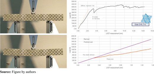
Set up on the machine for the physical tests of the specimens and graphic comparison between the numerical and real model referring only to the elastic part of the test
Set up on the machine for the physical tests of the specimens and graphic comparison between the numerical and real model referring only to the elastic part of the test
The results of the experimental tests and the comparisons with those expected from the numerical simulations are shown in Figure 10 together with some images of the different types of specimens used for the tests.
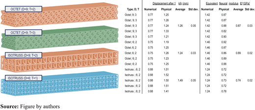
Representation of different types of specimens and comparison table between virtual and real simulations
Representation of different types of specimens and comparison table between virtual and real simulations
It was precisely in this phase of analysis that the greatest discrepancies between virtual and physical simulations emerged. The main factors related to the overestimation of the structural stiffness of numerical models are probably related to the fact that they are ideal. As well known, 3D printing causes voids and irregularities in printed material that are difficult to predict. The absence of a truly homogeneous material and the presence of layers that are not always perfectly interfaced with each other increase the divergence between the two models. The anisotropy of a printed model is another important factor. However, data obtained from the numerical tests are clearly proportional to the virtual estimated values (even if they represent worse mechanical behaviors and stiffnesses). This suggests that the ANOVA associated with the models works properly and that with further experimental evidence it is also possible to correctly map the behavior of the real system.
4. Conclusions
The virtual and experimental tests performed on the specimens have demonstrated the effectiveness of using continuous RSM for predicting the stiffness behavior of specimens subjected to three-point bending tests. The polynomial regression models accurately predicted stiffness, highlighting the ability of these nonlinear models to identify optimal design points that balance stiffness and lightness. However, limitations have been identified principally related to the physical tests. These are the anisotropic behavior of 3D-printed structures, the difficulties associated with 3D prototyping and the poor mechanical properties of polymer latex structures. These factors affect the validation of numerical models against real models and limit the industrial application of these structures. However, the authors identify the main success of the study in the fact that by integrating classical methodologies (ANOVA, RSM) with an effective parameterization of porous geometries it was possible to guide the design in a logical and optimal way. This included the possibility of choosing the optimal cell type by defining its dimensional parameters to ensure optimal ratios between weight and structural stiffness. This effort aims to reinforce the design principles inherent in lattice structures within the fields of scientific research and industrial production, which are still detached from theoretical research and focused on achieving functional models rather than optimal ones.
On behalf of all authors, the corresponding author states that there is no conflict of interest.
