Study on drying shrinkage and creep of manufactured sand concrete in railway prestressed structures

As of the end of 2024, China's total railway mileage in operation has surpassed 162,000 km, with high-speed railway accounting for 29.6% of the network. China's railway construction is progressively advancing into the challenging terrain of the western plateaus and mountains, with plans for further high-speed railway expansion in these regions (Wen et al., 2025). However, due to inefficient transportation and uneven resource distribution, the supply of concrete aggregates has emerged as a critical factor impeding railway construction progress and project quality (Gong, Ran, Bu, Xu, & Zhao, 2025). Against the backdrop of a global sand crisis where river sand (RS) is being extracted at a rate far exceeding its natural replenishment, the seasonal extraction patterns of natural RS and the implementation of extraction restriction policies have significantly exacerbated the shortage of critical aggregate resources in construction projects (Bendixen, Best, Hackney, & Iversen, 2019). Manufactured sand (MS), produced industrially in factories, is increasingly replacing RS as a green building material for concrete due to its cost-effectiveness, consistent quality and rapid production capabilities (Li et al., 2021). While extensive research exists on the quality control of MS and its impact on concrete's mechanical properties and durability (Shen et al., 2018; Yang et al., 2023), comparatively few studies have investigated the long-term deformation behavior of manufactured sand concrete (MSC), which limits the application of MS in high-strength railway prestressed structures including box girder, track slab and sleeper (Li et al., 2020).

Drying shrinkage and creep represent inherent time-dependent properties of concrete, directly governing structural deformation, and they are crucial for controlling cracks and calculating prestress loss in structural design (Zhu, Wang, Li, Zhao, & Huo, 2020; Zhang, Guo, & Xu, 2023). Empirical and semi-empirical models for characterizing the drying shrinkage and creep coefficients of river sand concrete (RSC), including the ACI model, fib MC 2010 model, GL 2000 model and B-series models (Silva, De Brito, & Dhir, 2015; Mastali, Kinnunen, Dalvand, Firouz, & Illikainen, 2018; Wendling, Sadhasivam, & Floyd, 2018; Abdalhmid, Ashour, & Sheehan, 2019; Huang et al., 2021), have been established in international standards based on extensive experimental data. The Chinese concrete design standard GB 50010–2010 specifies recommended values for drying shrinkage and creep, adapting formulas primarily derived from the European standard EN 1992–2. In contrast, the Chinese highway bridge code JTG 3362–2018 revises the CEB-FIP 90 model through calibration with empirical data from domestic engineering practices. Meanwhile, the railway standard TB 10092–2017 proposes shrinkage and creep parameters based on historical test data in the 1980s from the Southwest Institute of the China Academy of Railway Sciences. Critically, existing models and their calculated values in these standards are predominantly derived from RSC datasets. Consequently, their applicability to MSC structural design remains unverified and necessitates further validation.

MS produced by mechanical crushing and screening of rocks, differs from natural RS in its formation principle and exhibits distinguishing characteristics including diverse lithology, stone powder content and angular particles (Shen et al., 2016). These characteristics impart distinct long-term deformation behavior to MSC compared to RSC (Zhou, Wang, Zhu, & He, 2008). Early studies in the 1980s by Kourd et al. demonstrated that drying shrinkage of concrete increased proportionally with rock dust content (by mass of MS) (Bonavetti & Irassar, 1994; Goncalves, Tavares, Toledo Filho, Fairbairn, & Cunha, 2007). Conversely, Zhu et al. (2024) observed reduced drying shrinkage, lower crack sensitivity and enhanced crack resistance in MSC when incorporating ≤20% rock dust from diabase, tuff or basalt as mineral admixtures. Zhen et al. (2024) reported a 16.1% reduction in drying shrinkage by replacing 60%-80% RS with MS and adding moderate glass fibers. Liu et al. (2025) further reported that calcium carbonate crystals formed during carbonation curing filled transition pores and large capillary pores, thereby mitigating shrinkage cracking risks in MSC. Regarding creep behavior, Zhou et al. (2008) noted comparable creep coefficients between high-strength MSC (7% stone powder content) and RSC. Li, Wang, and Zhou (2009) observed higher compressive creep deformation in C60 MSC than RSC when stone powder content exceeded 7%. Long-term uniaxial compression tests by Li et al. (2022) revealed thicker interfacial transition zones (ITZ) and greater creep strain in MSC. Lithological variations in MS were also shown to influence MSC compressive strength, with higher strength correlating to lower creep under same stress conditions (Li et al., 2020). In summary, divergent findings persist regarding the drying shrinkage and creep behaviors of MSC, primarily attributed to variations in manufactured sand lithology, stone powder content, concrete strength grade and test methods. These inconsistencies impede reliable performance predictions for MSC in high-strength railway prestressed structures.

This study systematically investigates the drying shrinkage and creep behaviors of MSC, focusing on the effects of manufactured sand lithology and stone powder content. Nano-scratch characterization was employed to elucidate the microscale mechanisms by which MS influences concrete long-term deformation. Based on experimental results, prediction models for the drying shrinkage and creep coefficients of MSC were developed, incorporating the characteristics of MS. These findings aim to provide theoretical guidance and practical support for the application of MSC in high-strength railway prestressed structures.

In this study, concrete raw materials comprised cement, supplementary cementitious materials, fine aggregates, coarse aggregates, water and chemical admixtures. The cement (C) was ordinary portland cement with a strength grade of 42.5. The supplementary cementitious materials included fly ash (FA) and granulated blast furnace slag powder (SL). The key properties of these materials are summarized in Table 1. Fine aggregates comprised RS and four types of MS derived from tuff (TF), limestone (LS), basalt (BS) and granite (GN). These lithologies align with prevalent practices in Chinese railway engineering to ensure field relevance. To eliminate the influence of unrelated factors, all MSs were calibrated to identical gradation curves (fineness modulus = 2.8) and a uniform stone powder content of 5% through screening and secondary grading. The key properties of fine aggregates, compliant with the Chinese standard GB/T 14684–2022, are detailed in Table 2. Mineral compositions and surface micro-topographies are provided by Wang et al. (2024). Coarse aggregate was gravel (G), with a continuous grading ranging from 5 mm to 20 mm, which was employed for all concrete types. Chemical admixtures included a polycarboxylate-based superplasticizer (SP) and a rosin resin air-entraining agent (AE), whose dosages were adjusted to achieve comparable workability among concrete batches.

Concrete mixtures were formulated with varying lithological MSs (tuff, limestone, basalt, granite) and stone powder contents (0, 5%, 10%, 15%), and mix proportion design was conducted in accordance with the Chinese railway standard TB/T 3275–2018, as detailed in Table 3. For lithology studies, RSC served as the control group, while tuff (TFC), limestone (LSC), basalt (BSC) and granite (GNC) MSC were comparatively evaluated for drying shrinkage and creep behaviors. For stone powder content studies, tuff MS was selected to prepare MSC for its high strength and prevalence in railway engineering. MSC specimens with controlled stone powder contents (0%, 5%, 10%, 15% by MS mass) were produced through sieving and reconstitution, designated as TF0, TF5, TF10 and TF15, respectively. The slump of fresh concrete was targeted at (200 ± 20) mm, with entrained air content maintained at (3.5 ± 0.5) %.

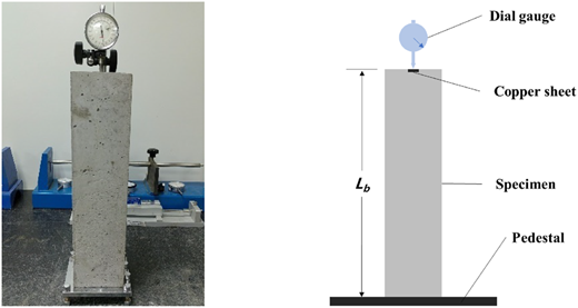
Drying shrinkage testing was conducted in accordance with Chinese standard GB/T 50082–2024. A copper sheet was pre-bonded to the base of a 100 mm × 100 mm × 400 mm prism mold. Fresh MSC mixtures were cast into the molds and demoulded after 24 hours. Specimens were then transferred to a standard curing chamber with (20 ± 2) °C and ≥95% RH for 3 days, followed by conditioning in a constant temperature-humidity laboratory with (20 ± 2) °C and (60 ± 5) % RH. As shown in Figure 1, a dial gauge was immediately mounted on the embedded copper sheet to initiate drying shrinkage measurements. Shrinkage strain was calculated using Eq. (1), with the mean value of triplicate specimens representing the drying shrinkage for each MSC group.

Where: $εst$ is drying shrinkage when test age of $t$ days (με, 1 με = 1 × 10⁻⁶); $L0$ is the initial dial gauge value (mm); $Lt$ is the dial gauge value when test age of $t$ days (mm); $Lb$ is the measurement gauge length which is the length of the specimen (mm).

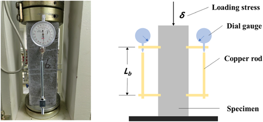
Compressive creep testing was conducted in accordance with Chinese standard GB/T 50082–2024. Four copper measurement points were pre-embedded in a 100 mm × 100 mm × 300 mm prism mold. Fresh MSC mixtures were cast into the molds and demoulded after 24 hours. Specimens were then cured under standard conditions for seven days, followed by conditioning in a constant temperature-humidity laboratory with (20 ± 2) °C and (60 ± 5) % RH. At 28 days of concrete age, copper rods were mounted on the pre-embedded measurement points, and dial gauges were installed on the rods to initiate compressive creep measurements, as shown in Figure 2. Three specimens per MSC group were loaded at a constant stress of 20 MPa, approximately 30% of the axial compressive strength of concrete. Additional three specimens were reserved for simultaneous drying shrinkage testing. Creep strain, specific creep and creep coefficient were calculated using Eq. (2)-(4), respectively.

Where: $εct$ is creep strain when loading age of $t$ days (με, 1 με = 1 × 10⁻⁶); $ΔLt$ is the total deformation value of concrete when loading age of $t$ days (mm); $ΔL0$ is the initial deformation value of concrete (mm); $Lb$ is the measurement gauge length which is 160 mm in this creep test; $εt$ is the drying shrinkage of the same age specimens (mm/m).

Where: $Ct$ is specific creep when loading age of $t$ days (MPa^-1); $δ$ is the loading stress which is 20 MPa in this creep test.

Where: $φt$ is creep coefficient when loading age of $t$ days; $ε0$ is the initial strain value during loading (με).

The MSC cube sample was sectioned into 15 mm × 15 mm × 5 mm specimens and mechanically polished. Nano-scratch testing was conducted using a Keysight Nano Indenter G200, comprising three sequential stages: Pre-scanning under 20 μN load to assess preliminary surface roughness; main scratch scanning under 50 mN load; post-scanning under 20 μN load to determine residual scratch depth. The indenter traversed at 4 μm/s, with three parallel scratches spaced 60 μm apart per specimen, each exhibiting a total scratch length of 200 μm. The test further enabled calculation of microfracture toughness at both the ITZ and the aggregate within the tested area, as defined in Eq. (5).

Where: $Rc$ is the microfracture toughness (MPa·m^-0.5). $FT$ is the tangential load (mN). $d$ is the scratch depth (μm). $ld$ is the edge length of the measured volume (μm). $Ad$ is the projection of the measured volume on the plane perpendicular to the direction of the scratch (μm²), $ldAd=2.2808d3$ (Wei, Kong, Wang, & Sha, 2021).

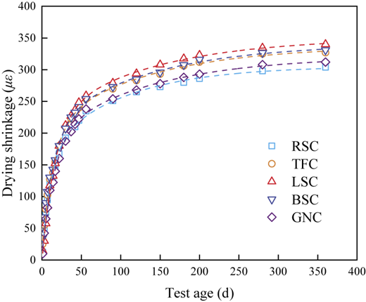
Figure 3 presents the drying shrinkage evolution of MSC with varying lithologies. The shrinkage development pattern of MSC closely aligns with that of RSC, exhibiting a characteristic two-stage behavior: a significant increase before 56 days of age, followed by markedly slower growth thereafter. This phenomenon primarily stems from the superposition of two mechanisms: migration and dissipation of adsorbed water driven by hydrostatic tension in capillary pores, and ongoing hydration of cementitious materials (Zhang, Zakaria, & Hama, 2013). During the early stage of hardening, internal higher humidity of fresh concrete accelerates moisture loss and hydration kinetics (Mastali et al., 2018; Ocak, Bekdaş, Isikdag, Nigdeli, & Bilir, 2024), resulting in pronounced shrinkage. As internal humidity progressively decreases and hydration stabilizes, the shrinkage rate gradually diminishes. Consequently, drying shrinkage manifests rapid initial development that transitions to asymptotic stabilization over time.

Except for MS lithology and polycarboxylate superplasticizer dosage, the factors influencing drying shrinkage, including water-to-binder ratio, aggregate gradation, cement dosage, mineral admixtures, component size and curing conditions, were uniformly controlled. The 360 days drying shrinkage for RSC, TFC, LSC, BSC and GNC were 304 με, 327 με, 340 με, 331 με and 312 με, respectively. Two factors contribute to the higher drying shrinkage of MSC compared to RSC. (1) Reduced aggregate volume fraction: With identical fine and coarse aggregate contents, the 5% stone powder content in manufactured sand reduces aggregate volume fraction in MSC, diminishing its shrinkage-inhibiting effect (Zhang et al., 2013). (2) Lithology-dependent water absorption: Variations in manufactured sand lithology significantly affect water absorption (Table 1), requiring adjusted superplasticizer dosages to achieve comparable workability. Higher water absorption necessitates greater superplasticizer dosage. Superplasticizer refines capillary pores and increases internal water content (Fu, Xia, Xu, Zhang, & Jia, 2022). Finer, more uniform capillary pores generate higher negative pressure during dehydration, amplifying MSC shrinkage.

Notably, LSC exhibits marginally higher shrinkage than other MSC types. Limestone powder accelerates hydration by nucleating calcium hydroxide and C-S-H formation while reacting with C₃A to form hydrated calcium aluminate (Bentz et al., 2015), increasing hydration products and thus cement paste shrinkage. All high-strength MSC specimens exhibited 56 days drying shrinkage below 400 με, complying with the Chinese railway standard TB/T 3275–2018. This confirms the feasibility of utilizing diverse lithological manufactured sands in railway prestressed structures.

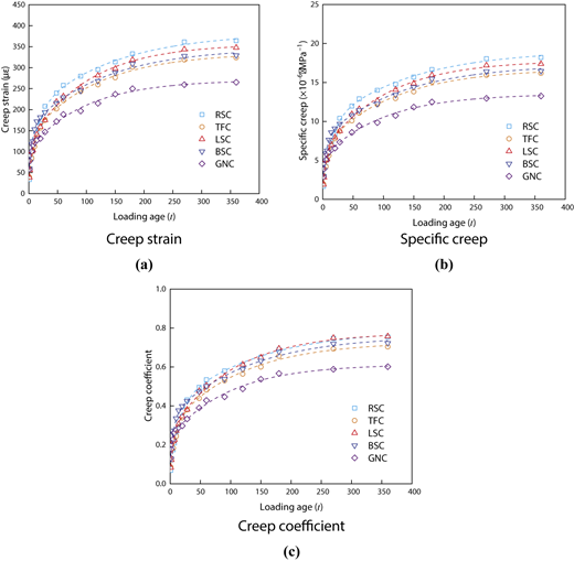
Figure 4 presents the creep strain, specific creep and creep coefficient of MSC with varying lithologies. The creep development trends of MSC align with those of RSC, exhibiting accelerated strain progression before 28 days of loading age and decelerated growth thereafter. As shown in Figure 4(a), the 360 days creep strains for RSC, RSC, TFC, LSC, BSC and GNC measure 364 με, 324 με, 348 με, 330 με and 265 με, respectively.

Creep strain, defined as the time-dependent deformation of concrete under sustained load, is influenced by complex factors including raw materials, mix proportion, environmental conditions, load characteristics and structural dimensions (Silva et al., 2015). In this experiment, lithological variations in MS altered the mechanical properties of MSC due to differences in aggregate strength and surface texture. As evidenced by the compressive strength and crushing index data in Table 2, combined with surface roughness measurements from Wang et al. (2024), the comprehensive strength ranking of MSC is GNC > TFC > BSC > LSC > RSC, as shown in Table 3. Higher strength concrete exhibits superior resistance to stress-induced microcracking at the aggregate-paste interface. This inhibits gel particle sliding and consolidation triggered by water molecule rearrangement in cementitious pores, thereby suppressing basic creep (Shariq, Prasad, & Abbas, 2016).

Specific creep is the creep deformation of concrete under unit stress and creep coefficient is the ratio between the creep compression and the initial deformation value under loading. As shown in Figure 4 (b) and (c), the variation law of specific creep and creep coefficient of railway high-strength MSC is consistent with creep strain. The specific creep remains ≤25 × 10⁻⁶ MPa^-1, while the creep coefficient is < 1.0. These values demonstrate that MSC prepared with high-quality MS possesses exceptional creep resistance.

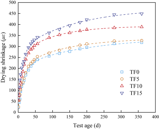
Figure 5 presents the drying shrinkage of MSC with varying stone powder contents. At 360 days, the drying shrinkage values for TF0, TF5, TF10 and TF15 are 318 με, 327 με, 389 με and 449 με, respectively. Drying shrinkage exhibits a positive correlation with stone powder content. This trend arises because increased stone powder content elevates the powder volume fraction while reducing the aggregate volume fraction in concrete, thereby diminishing the aggregate's constraint on shrinkage deformation.

Notably, TF15 shows a significant 41.2% increase in drying shrinkage compared to TF0. This is attributed to the additional 110.25 kg of powder material per cubic meter, which reduces internal constraint forces and amplifies shrinkage strain. Conversely, the drying shrinkage increment of TF5 is only 2.8%. This suggests that an optimal stone powder content enhances concrete compactness through pore-filling effects, inhibiting internal moisture evaporation under dry conditions (Mu, Li, Lin, Liu, & Luo, 2023). The filling effect partially counteracts the adverse impacts of reduced aggregate volume fraction.

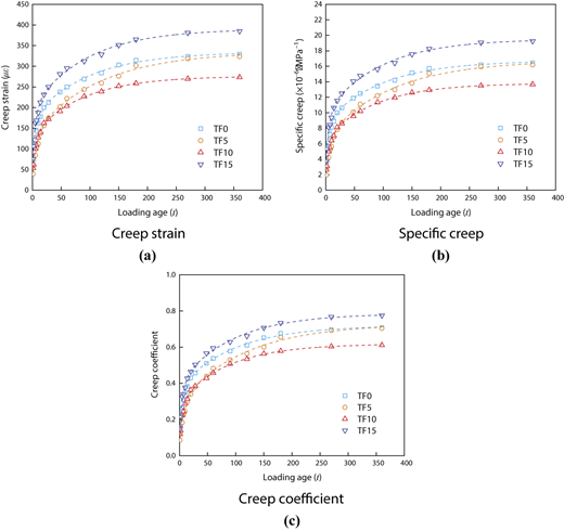
Figure 6 presents the creep strain, specific creep and creep coefficient of railway high-strength MSC with varying stone powder contents. Significant differences in creep behavior are observed across specimens: at 360 days loading age, creep strains for TF0, TF5, TF10 and TF15, are 324 με, 324 με, 249 με and 385 με, respectively. Creep strain exhibits a nonlinear trend with increasing stone powder content, initially decreasing before rising substantially at 15% content. Notably, TF10 demonstrates the minimum creep strain.

Macroscopically, the compressive strength hierarchy follows TF10 > TF5 > TF0 > TF15. Enhanced strength due to stone powder's filling effect improves concrete's resistance to creep deformation. Microscopically, optimal stone powder content refines cement paste packing density and elevates concrete compactness, as validated in prior studies (Wang, Li, Huang, Yi, & Yang, 2023). However, excessive inert stone powder (>10%) dilutes cementitious matrix cohesion, reducing strength and facilitating nanoparticle sliding within C-S-H gel under sustained load (Silva et al., 2015), thereby amplifying creep strain. Considering the combined effects on drying shrinkage and creep, the stone powder content in MS should be limited to ≤10% for railway MSC applications.

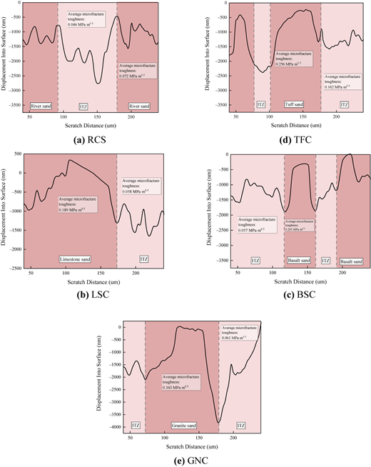
The enhanced resistance of MSC to creep is attributed to the superior hardness of manufactured sand aggregates and their optimization of the ITZ. As depicted in Figure 7, nano-scratch tests near fine aggregates reveal that scratch depth in aggregates is significantly lower than in the ITZ across MSC with varying lithologies. This confirms that fine aggregates provide skeletal support within the concrete matrix, endowing MSC with a higher elastic modulus (He et al., 2025). The microfracture toughness of MSC is higher than that of RSC. Specifically, the average microfracture toughness of RSC is 0.072 MPa·m^0.5 while those of TFC, LSC, BSC and GNC are 0.256 MPa·m^0.5, 0.189 MPa·m^0.5, 0.205 MPa·m^0.5 and 0.343 MPa·m^0.5, respectively. These results indicate that higher aggregate hardness more effectively inhibits stress-induced microcrack initiation and optimizes skeletal support.

In contrast to RSC, MSC significantly enhances the properties of the ITZ, as demonstrated in Figure 7. The average fracture toughness of RS at the ITZ is 0.046 MPa·m^0.5, while near TF, LS, BS and GN, its average microfracture toughness values are 0.162 MPa·m^0.5, 0.058 MPa·m^0.5, 0.057 MPa·m^0.5 and 0.061 MPa·m^0.5, respectively. The higher water absorption of MS reduces the effective water-to-binder ratio within its ITZ compared to RSC. Furthermore, the incorporation of stone powder densifies the ITZ microstructure, endowing the MSC aggregate interface with superior fracture toughness. Notably, TFC exhibits the highest fracture toughness, attributed to tuff's unique composition as a compacted pyroclastic rock rich in feldspar and metakaolin. This composition enhances interfacial cohesion through microstructural characteristics derived from volcanic activity (Zhang, Lu, Liu, Wang, & Ge, 2024).

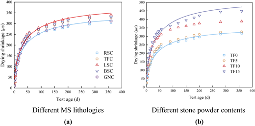
The temporal evolution patterns of drying shrinkage and creep in MSC closely align with those of RSC. However, divergent ultimate deformations arise due to the distinct properties of MS. Based on the prediction model specified in Chinese standards, modified drying shrinkage models for MSC are formulated through Eq. (6) to (9), incorporating a dimensionless correction factor a. This factor quantifies the synergistic effects of MS lithology and stone powder content. Figure 8 illustrates the strong agreement between predicted and experimental drying shrinkage values for MSC, while Table 4 details the corresponding model parameters. The high correlation coefficients (R² > 0.95) confirm the model's accuracy and applicability for engineering practice.

Where: $εcs(t)$ is the calculated drying shrinkage when test age of $t$ days; $a$ is the correction factor of drying shrinkage; $βsc$ is a coefficient determined based on the cement type, and it is 5.0 for general Portland cement or rapid hardening cement; $fcm$ is 28 days compressive strength of concrete (MPa); $RH$ is annual average relative humidity of the environment (%); $h$ is the theoretical thickness of components (mm), $h=2A/u$⁠, $A$ is the component cross-sectional area and $u$ is the peripheral length of the component in contact with the atmosphere; $fcm0$ = 10.0 MPa; $RH0$ = 100%; $h0$ = 100 mm.

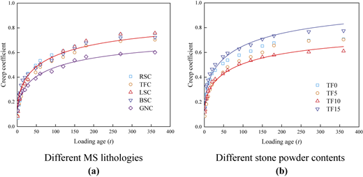
Prediction models for the creep coefficient of MSC are formulated through Eq. (10) to (15) by introducing a dimensionless correction factor b. The computational results of these models are presented in Table 5 and Figure 9. The high correlation coefficients (R² > 0.95) validate the models' capability to accurately predict the creep coefficient of MSC, thereby supporting the design and application of MSC in railway prestressed structures.

Where: $φ(t,t0)$ is the calculated creep coefficient when test age of $t$ days; $t0$ is the age of concrete during loading (d); $b$ is the correction factor of creep; the other parameters are the same as those in the drying shrinkage prediction models.

The study aims to understand the drying shrinkage and creep behavior of MSC with varying lithologies and stone powder contents. The following conclusions can be drawn based on the experimental results:

1. The drying shrinkage of MSC exceeds that of RSC, yet its creep resistance is superior, and high-quality MS should be preferred in the preparation of low-deformation MSC. The higher aggregate hardness of MS inhibits stress-induced microcrack formation, thereby reducing gel particle sliding and consolidation triggered by water molecule rearrangement in cementitious pores. However, the reduction of aggregate volume fraction and increase of superplasticizer dosage increase drying shrinkage of MSC.

2. Drying shrinkage increases monotonically with stone powder content, whereas creep strain follows a nonlinear trajectory – decreasing initially before rising significantly beyond 10% content. To achieve both low shrinkage and low creep of MSC, the stone powder content of MS is recommended to be ≤ 10%.

3. The established prediction models (incorporating correction factors for lithology and stone powder content) accurately characterize drying shrinkage and creep coefficient evolution in MSC. These models provide critical design parameters for MSC applications in railway prestressed structures.