International Environmental Agreements and Trading Blocks — Can Issue Linkage Enhance Cooperation?

Environmental problems such as global warming, ozone depletion and acid rain are transboundary or global in nature, that is, a single country’s unilateral actions cannot yield significant improvements. The effective response to such problems necessitates the formation of international agreements, in which participation has to be voluntary, given the absence of an international environmental authority.

Voluntary participation in agreements involving global public goods is very small as both recent experience and the theoretical literature show. Therefore, providing countries with incentives to participate in global environmental agreements is of paramount importance for sustaining large coalitions, able to tackle serious environmental problems. In this paper we examine whether a joint trade and environmental agreement could provide countries with incentives such that a successful agreement is formed. In particular, we consider a joint agreement under which, member countries trade freely among themselves, charge a common tariff to imports from non-members and levy a common tax on members’ emissions. We find that membership to such an agreement is substantially larger compared to an agreement on just a common environmental policy. We show, using numerical simulations, that participation improves at a rate of around seventy percent, and that these large coalitions are also achieving substantial welfare improvements.

It is interesting to note that some existing International Environmental Agreements (IEAs) include provisions that affect trade. The intentions of such provisions are mainly three: to monitor and control, or even completely ban trade in certain materials or products; to comply with the IEA’s requirements and to provide the means of enforcing environmental targets, by imposing trade sanctions on non-members. For example, the Montreal Protocol contains specific trade measures in the form of requirements for a ban on trade between parties and non-parties in products containing or made with ozone-depleting substances. The strategy of linking participation in the Protocol to trade sanctions proved to be successful according to reports which state that a number of the countries joined the treaty because of the trade provisions (Brack and Gray, 2003). Moreover, trade sanctions have been utilized in the Basel Convention (international transportation of hazardous waste), and the Convention on International Trade in Endangered Species (CITES). With respect to a specific product, the U.S. has applied a penalty tax on foreign automobile manufacturers not meeting the domestic Corporate Average Fuel Economy (CAFE) standards.

The above mentioned agreements belong to a large group of agreements that attempt to control specific environmental and natural resource problems that are global in nature. The IEAs’ effectiveness in dealing with the respective environmental problem varies. The Montreal Protocol is a well sited example of a very successful IEA, eliminating the production of ozone-depleting substances. Other agreements, such as the ones on climate change, namely the Kyoto Protocol and its successor the Paris Agreement, are not as successful because either they do not set ambitious enough targets, or, if they do, they attract limited participation. As already mentioned, free-riding incentives emerging from the pure public good nature of the environmental issues, prevent the attainment of large welfare gains associated with increased cooperation to ambitious agreements.

The main body of the literature studies the formation of an IEA as a two-stage non-cooperative game, where in the first stage countries decide whether to join the coalition or not, while in the second stage they choose their emissions’ level. The subgame perfect Nash equilibrium of the resulting two-stage game is derived by applying the notions of internal and external stability conditions as introduced by D’ Aspremont et al. (1983)¹ The literature examining the above problem, assuming that countries choose emissions in the second stage either simultaneously² or that the coalition acts as a leader,³ concludes that strong free-rider incentives prevent large stable coalitions and/or large gains from cooperation.

Given these pessimistic results, the literature has provided a number of suggestions to improve participation in IEAs. The most prominent proposals refer to direct transfer payments by coalition members and to linking participation in the IEA to other issues such as trade agreements, in order to attract new members into the coalition. The intuition behind the latter proposal is to link the environmental game, in which members of the IEA cannot exclude non-members from enjoying the benefits that the IEA generates, to a club good game where exclusion from enjoying the club benefits is possible.

A substantial literature on issue linkage has developed following the original contributions by Folmer et al. (1993) and Folmer and van Mouche (1994) that consider both multiple isolated one-shot games and repeated games and show that connecting environmental with trade agreements improves the possibility of cooperation. Barrett (1997) analyzes an IEA formation problem in a partial equilibrium model with abatement and illustrates that trade sanctions can help to support cooperation, even full cooperation, among countries. Carraro and Marchiori (2004) consider two isolated games, an environmental agreement game and a trade agreement game, and introduce an initial stage at which countries decide whether to link negotiations of the two games. They find that countries decide to link the two games only if benefits from large environmental coalitions are substantial. Lessmann et al. (2009) apply a dynamic model of climate coalition formation and use trade sanctions as an instrument to promote participation. In their model, coalitions are free to impose tariffs on imports from non-cooperating countries. They find that participation in the coalition increases and so does global welfare. More recently Nordhaus (2015), employing a numerical general equilibrium model, introduces exogenously determined tariff sanctions to encourage participation in climate agreements. He finds that trade penalties on non-participants induce a large stable coalition with high levels of abatement. An extensive review of the IEAs literature including issue linkages is provided by Marrouch and Chaudhuri (2016), while Maggi (2016) reviews issue linkage in international cooperation including environmental agreements.

The present paper contributes to this literature by considering a joint environmental and trade agreement as described above. In such an agreement, signatories on the one hand enjoy the benefits of tariff-free access to other signatories’ markets and on the other hand bare the burden of a high tax on emissions. In contrast, nonsignatories weight the benefits of charging a lower emission tax, free riding on signatories’ environmental efforts, to the costs of being excluded from the free-trade area. The main objective of the paper is to examine the effect that the inclusion of trade sanctions has on the level of participation and the effectiveness of such a joint international agreement in improving welfare.

We assume that there is one single firm in each country producing a homogeneous good that emits a harmful, global pollutant. Firms sell their production to the local and the foreign markets, forming a global Cournot oligopoly. Countries maximize their welfare taking into account the damages from global pollution. Decisions are taken in the following three stages: first, each country decides whether to join the agreement; second, countries choose simultaneously — the signatories cooperatively and the nonsignatories non-cooperatively — the tariff and tax levels; in the third stage, each firm, taking countries’ and other firms’ choices as given, maximizes its profits. To obtain the subgame perfect Nash equilibrium, the model is solved by backward induction.

The main result of this paper is that a joint environmental and trade agreement, substantially improves participation relative to the situation in which the agreement involves only environmental policies. Furthermore, increased participation also yields substantial welfare benefits. Although the paper does not provide analytical proofs, numerical simulations indicate that trade sanctions yield two stable coalition sizes. The smaller stable coalition although it can contain up to 48% of the total number of counties yields very small welfare improvements. The larger stable coalition contains consistently 70% of the total number of countries and provides substantial welfare improvements of around 60% of the welfare improvement the grand coalition attains over the smallest possible coalition of two countries. These results definitely present a great improvement over the grim prediction of a coalition of up to two members associated with small welfare improvements regardless of the number of countries.

The framework used in the present paper relates closer to the recent work by Eichner and Pethig, since they also assume that countries trade and they can form an agreement on a common environmental policy. Contrary to our framework that allows for tariffs, they assume free trade and thus, they do not consider joint trade and environmental agreements. They instead examine the effect that free trade among countries has on the size of the coalition relative to autarky. Assuming a cap and trade policy and that countries choose simultaneously, Eichner and Pethig (2014) find that participation in the agreement does not improve, while if the coalition behaves as a Stackelber leader, Eichner and Pethig (2013) find that participation increases but without any significant welfare improvements. If the policy instrument is a tax on emissions, Eichner and Pethig (2015) demonstrate that even the grand coalition is stable under some conditions which though require small emission reductions. The main difference between the above papers and our work is that Eichner and Pethig examine the effect of free international trade on coalition formation while we focus on the effect of a joint trade and environmental agreement on the size of the coalition and welfare.

The rest of the paper is structured as follows. Section “The Model” describes the model. Section “Two Benchmark Cases” presents two benchmark cases: the Nash and the full cooperation. Section “Coalition Formation” examines the formation of a joint environmental and trade agreement. Section “The Stability of an Agreement” presents the stability conditions, while Section “Numerical Analysis” discusses the effect of allowing for joint trade and environmental agreements on the size of the coalition and on aggregate welfare. Since analytical results are impossible to derive, we resort to numerical simulations and we provide robustness tests for the model’s variables. Section “Conclusions” concludes the paper.

We consider an open economy consisting of n identical countries, N{1, 2, . . . , n}. There is one single profit maximizing firm located in each country producing quantity $eip$ of good e. Firms form an international oligopoly, choosing quantities simultaneously. The literature on oligopoly in international trade, dating back to Brander (1981) and Brander and Krugman (1983), has shown that intra-industry trade of homogeneous products exists.⁴ In order to focus on the issue of environmental negotiations, we simplify our model by assuming that e is a homogeneous product. We further assume that there are no costs of exporting and thus, each firm sells its production in its home market as well as in the foreign markets. Thus, country i’s production, $eip$⁠, is the sum of domestic consumption of own production, $eid$⁠, and exports to all other countries j ∈ N and j ≠ i, denoted by $eijX$⁠,

The representative consumer in each country i ∈ N has a utility function of the form,

where $eic$ is country i’s total consumption of the traded good, K_i denotes consumption of a numeraire good, and a > 0 and b > 0. The numeraire good is produced under perfect competition with constant returns to scale. The commonly used quasi-linear utility function rules out income effects. Total consumption in country i, $eic$⁠, is given by,

where $eid$ is country i’s consumption of the domestically produced good by firm i, and $eijI$ indicates the quantity country i imports from country j ≠ i (i.e., quantity exported from country j to country i).

Maximization of the utility function, Equation (2), yields country i’s inverse demand function for the good e,

If trade does not occur, that is, $eijI$⁠, ∀i, j ∈ N, then $eic=eid=eip$⁠, which implies that each national market is served by a domestic monopoly. In the case of international trade that we consider, $eic≠eid≠eip$⁠.

We assume that production of good e generates emissions of a global pollutant. To keep the model tractable, we assume that all firms operate with the same technology implying a linear relationship between production and emissions. In particular, we assume that one unit of production results in one unit of emissions, which implies that total pollution is $E=∑i=1neip$⁠. The damage from pollution is monotonically increasing and convex in the global emissions, E. In particular, the damage function is given by,

where c > 0, and D_i (0) = 0, $Di′≥0$⁠, and $Di″>0$⁠. Furthermore we assume that there is no pollution associated with the production of the numeraire good.

Countries could intervene to both promote their domestic firm’s interests in international trade and reduce damages from emissions. They can attempt to achieve these goals by either taking unilateral actions or acting collectively by forming a trade and environmental agreement. We consider that country i’s unilateral trade policy instrument is a nonnegative tariff, at the rate of τ_i per unit of import from all other countries j, where j ≠ i. Country i’s environmental policy instrument is a carbon tax t_i per unit of domestic emissions, which, by assumption, equal domestic production. Alternatively, countries could choose both policy instruments collectively, forming a coalition that signs an agreement on a common set of {τ, t}. With respect to the nature of the two issues it should be noted that the global aspect of pollution makes environmental negotiations very difficult since, as a public good game, they involve strong free-riding incentives. On the other hand, trade negotiations, as a club good game, are more straight forward.

We model the process of countries’ decision with respect to trade and environmental policy as a non-cooperative three-stage game. We use the equilibrium concept of subgame perfect Nash equilibrium and we start from the last stage, at which, taking countries’ decisions as given, firms simultaneously choose quantities (Cournot). In the second stage, countries choose simultaneously, either unilaterally or cooperatively, tariff and emission tax levels. In the first stage, each country decides whether or not to join the coalition.

In the third stage of the game, firms choose simultaneously the quantity of e that will produce and sell to the domestic market, $eid$⁠, and export to each of the foreign markets, $eijX$⁠. Each firm maximizes profits, taking the policies set by the countries and the output decisions of the other firms as given. For simplicity, the marginal cost of production is assumed to be constant and equal to zero. Firm i is charged an emission tax t_i per unit of $eip$⁠. In addition, firm i’s effective marginal cost of exporting to country j is τ_j and similarly, firm j’s effective marginal cost of exporting to country i is τ_i. The total profits for the firm located in country i consist of the profits from sales in the domestic market i plus the profits from sales in country j, minus the pollution tax imposed on its emissions,

Firm i maximizes profits, given by Equation (6), by choosing quantity sold in country i, i.e., $eid$⁠, and quantity sold in country j, i.e., $eijX$⁠, for all j ≠ i ∈ N. Given the assumption of zero marginal cost of production and that the effective marginal cost of exporting to country j is τ_j, firm i’s profit maximization problem is,

We substitute demand $pi(eic)$ from Equation (4) and total consumption $eic$ from Equation (3) into firm i’s profit. We also note that due to symmetry, imports to country i from all other countries are equal and thus,$∑j≠ieijI=(n−1)eijI$⁠. Then, the first-order condition of Equation (7) with respect to $eid$ yields $eid$ as a function of $eijI$⁠,

Furthermore, we take into account that the quantity exported from country i to country j equals the quantity country j imports from country i, that is $eijX=ejiI$⁠, and that $∑i≠jejiI=∑k≠j,iejkI+ejiI=∑k≠j,iejkI+eijX$ with $∑k≠j,iejkI=(n−2)ejkI=(n−2)eijX$⁠. Then, the first-order condition of Equation (7) with respect to $eijX$ yields $eijX$ as a function of $eid$⁠,

Due to symmetry, we can deduce the quantity country i imports from country j, using Equation (9), $eijI=ab−τi−tj−beidnb$⁠. Substituting this into Equation (8) yields domestically consumed own production $eid$⁠,

Symmetry allow us to infer $eid$ from Equation (10), which we then substitute into Equation (9) to derive country i’s exports to country j,

Again due to symmetry we can deduce from the above the quantity of imports,

Finally, we can substitute the above into the definition of $eic$ in Equation (3) to derive domestic consumption,

Consider the case that all countries, being symmetric, choose the same tariff τ_i = τ_j = τ, and emission tax t_i = t_j = t. In such a case, $eid(t,τ)=ab−t+(n−1)τ(n+1)b$ while $eijX(t,τ)=eijI(t,τ)=ab−t−2τ(n+1)b$ and $eic=eid(t,τ)+(n−1)eijI(t,τ)=abn−nt−(n−1)τ(n+1)b$⁠. Furthermore, notice that in the case of no policy intervention, t = τ = 0, $eid=eijX=eijI=eicn=na(n+1)$⁠. In the case of absolute symmetry and without policy intervention, the demand for the homogeneous good in each country $eic=na(n+1)$ is covered by equal amounts $a(n+1)$ from each one of the n firms. Each firm produces $eip=na(n+1)$⁠, sells $1n$ of that locally and exports an equal amount to the rest of the n − 1 countries. These results are in accordance with the theory on intra-industry trade in homogeneous products (cross-hauling), given that countries have the same preferences, firms have symmetric constant or zero marginal cost of production and zero transportation costs.⁵ When countries impose identical tariffs on imports τ > 0 and emission taxes on domestic production t > 0, domestic sales of the local firm exceed imports from (or exports to) another country, $eid>eijX=eijI$⁠. This is due to the fact that local sales do not face tariffs and that is why the difference between local sales and exports to another country increases with the tariff, $eid−eijX=τb$⁠. A tariff prevents, to a certain extent, penetration of foreign firms into the local market despite the fact that is set at the same level by all countries. On the contrary, the emission tax does not generate any differentiation since it is levied on total production.

In the second stage of the game countries choose the level of their policy instruments, after deciding in the first stage whether they will do it jointly with other countries or unilaterally. We will set up countries’ welfare here and we will examine their choices in the next sections. We assume that firms’ profits and countries’ revenues from tariffs and environmental taxes are rebated back to consumers. So that, country i’s welfare, denoted by W_i, consists of the domestic consumer surplus CS_i,⁶ the domestic firm’s profits Π_i(net of all taxes), the tariff revenues T R_i, the emission tax revenues ER_i and the environmental damages due to the aggregate pollution level D_i(E). That is,

Thus, country i’s total welfare can be written as,

where the quantity $eijX$ indicates country i’s exports to country j while the quantity $eijI$ indicates country’s i imports from country j.

The solution of the third-stage problem, specified above, provides firm i’s choice variables as functions of the policy parameters in country i and all other countries j ≠ i. Substituting these expressions into Equation (15) we obtain country i^′s welfare as function of policy parameters in all countries,

We will use Equation (16) to derive countries’ optimal choices first in two cases that the countries’ decision on whether to join the coalition is exogenously determined and then in the case that the first-stage decision is endogenously determined. The first two cases define the two extreme benchmarks against which the endogenously determined coalition will be compared to.

The following two cases are examined: in the first we assume that in the first stage all countries choose unilaterally the level of both policy instruments; in the second we assume that all countries choose jointly the level of both policy instruments.

The assumption of unilateral action means that in the second-stage country i chooses tariff and emission tax levels by maximizing Equation (16), taking all other countries’ choices of tariff and emission tax levels as given,

The first-order conditions for the above welfare maximization problem yield two reaction functions expressing country i’s policy choice variables τ_i and t_i as functions of country j’s policy choice variables, that is, τ_i(τ_j, t_j) and t_i(τ_j, t_j). Since countries are identical, both the tariff and the pollution tax will be the same in all countries. Imposing τ_nc = τ_i = τ_j and t_nc = t_i = t_j in country i’s reaction functions, yields τ_nc(t_nc) and t_nc(τ_nc). The subscript nc denotes the equilibrium value of variables in the non-cooperative case. It is clear from the solution that is presented in Appendix A, that $∂τnc∂tnc<0$ and $∂tnc∂τnc<0$⁠; that is, an increase in any of the two policy tools affects negatively the other.

We derive the equilibrium values of the tariff and the environmental tax by solving τ_nc(t_nc) and t_nc(τ_nc). The equilibrium values of the tariff and the environmental tax are,

and

respectively, where X = 2n − 1 and Ψ = 3n + Xnγ − 2. In order to simplify the presentation of the results, we define parameter γ as the ratio between environmental damages and benefits from emissions, that is, $γ=cb$⁠.

We can now substitute the equilibrium values of the tariff and the environmental tax into Equations (10) and (13) to derive the equilibrium choices of firms and consumers. The domestically produced and consumed quantity is

The quantity imported from any country equals the quantity exported to any country,⁷

Total quantity consumed in any country equals total domestic production,

Given the assumption of absolute symmetry among countries, it can be easily verified that $encc=encd+(n−1)encI$⁠. Given symmetry, aggregate consumption equals aggregate production and therefore the aggregate pollution level is

We can now derive countries’ welfare in the case of non-cooperation, as function of the model’s parameters,

The Cournot equilibrium with trade among countries that we examined above does not yield the same results as in Rubio and Casino (2001). Since in our model countries impose positive tariffs, each country’s production is lower and thus, total production and emissions are lower.⁸ It should be noted that if we allowed for free trade, that is, countries were setting τ_nc = 0, while choosing unilaterally t_nc, total production and thus emissions would exceed those reported in Rubio and Casino (2001).⁹

Assuming full cooperation implies that countries abolish tariffs and set a common emission tax level which maximizes their aggregate welfare. Therefore, in the second-stage countries choose the emission tax level by maximizing the sum of their welfare given in Equation (16), after setting τ_i = τ_j = 0 and t_i = t_j = t_c, where the subscript c indicates the full cooperation equilibrium values. That is,

The first-order condition of the above problem yields the common emission tax level,

Substituting the common emission tax into Equations (10) to (13), we derive the equilibrium choices of firms and consumers. Note that as expected from the discussion at the end of Section “Firm’s Choices”, we get $ecd(tc,tc,0)=ecX(tc,tc,0)=ecI(tc,tc,0)=ab−tc(n+1)b=ec.$⁠. Since tariffs are abolished under full cooperation, there is nothing to differentiate between local sales and exports. This implies that total quantity consumed in each country equals total quantity produced, $ecc=ecp=nec$⁠. Substituting the value of the emission tax from Equation (26) yields,

Aggregate production and thus emissions is,

Country i^′s welfare as function of the model’s parameters in the case of full cooperation is,

From the above derived solutions we can compare the two benchmark cases. From Equations (23) and (28) it is easily checked that E_nc > E_c and from Equations (24) and (29) that $Wc>Wnc, for γ>1nX$⁠. Thus, it is verified that in the case of full cooperation, aggregate emissions are lower and each country’s welfare higher relative to the Nash equilibrium.

Note that since in full cooperation tariffs are eliminated, the derived solutions for the total emissions and welfare are equivalent to the solutions presented in Rubio and Casino (2001). The optimally chosen emission tax leads firms to the same level of output as that chosen at the country level in Rubio and Casino.¹⁰

We now turn to endogenize the choice in the first stage of the game. That is, each country decides whether to join a group of countries, formally signing a legally bidding agreement specifying the level of the tariff and the emission tax, or choose the values of t and τ unilaterally. We call the former countries signatories to the agreement and we denote their variables with a subscript s. The rest of the countries acting as singletons are called nonsignatories and we denote their variables with a subscript ns. On the trade side, the agreement eliminates tariffs among signatories, while they levy a tariff τ_s on imports from nonsignatories. Nonsignatories levy a positive tariff τ_ns on imports from both signatories and other nonsignatories. On the environmental side, signatories choose a common emission tax t_s that maximizes the sum of the coalition’s welfare, while nonsignatories choose unilaterally their emission tax t_ns.

In particular, we assume that a set of countries S ⊂ N sign the agreement and the remaining N\S countries do not. Members of the coalition of size s = |S|, act cooperatively maximizing their aggregate welfare, while the remaining (n − s) nonsignatory countries act non-cooperatively maximizing their own welfare. Taking advantage of the symmetry assumption, we treat all signatory countries as equals within the coalition.

Given that we now have two groups of countries, signatories and nonsignatories, we have to calculate the following set of ten variables: consumption of domestically produced good, $esd$ and $ensd$⁠, imports within each group, $essI$and $ensnsI$⁠, imports across the two groups, $esnsI$ and $enssI$⁠, exports within the group, $essX$and $ensnsX$⁠, and finally exports across the two groups, $esnsX$and $enssX$⁠. The first element of a double subscript on imports (exports) indicates the group to which the importing (exporting) country belongs, while the second element the group to which the exporting (importing) country belongs. We note, as in the previous section, that imports from country i to j equal exports of country j to i, where i, j = s, ns, which implies, $essI=essX,ensnsI=ensnsX$⁠, $esnsI=enssX$ and $enssI=esnsX$⁠. We also note that since signatory countries eliminate tariffs among themselves and set a common emission tax, $esd=essI=essX$⁠. On the other hand though, $ensd≠ensnsI=ensnsX$⁠, since nonsignatories levy tariffs on imports from other nonsignatory countries. Thus, we have to specify five variables at the equilibrium, using the respective first-order conditions of signatory and nonsignatory countries’ profits.

Next, we define consumption in each group. A signatory country’s total consumption of e is given by,

Similarly, a nonsignatory country’s total consumption is,

To derive consumption and production choices, as functions of the policy parameters we use the first-order conditions of the firms’ profit maximization in each group. Rewriting Equation (7) to take into account the presence of two groups of countries, firms in the signatory and nonsignatory countries solve,

and

respectively.

Solving the first-order conditions, with respect to the five choice variables, yields domestic production, imports and exports for each signatory and nonsignatory country as functions of the policy parameters. For a signatory country, these quantities are,

The respective variables for a nonsignatory country are,

From Equations (34) and (38) it is clear that an increase of the tariff signatories levy on imports from nonsignatories will support domestic sales and trade among members of the coalition, $∂esd∂τs>0$⁠, to the detriment of imports from nonsignatories, $∂esnsI∂τs<0$⁠. Since we are expecting the environmental coalition to charge a higher emission tax, i.e., t_s > t_ns, we show that the larger the difference t_s − t_ns is, the smaller are domestic sales and trade among members of the coalition, $∂esd∂(ts−tns)<0$⁠, benefiting imports from nonsignatories, $∂esnsI∂(ts−tns)>0$⁠.

Domestic sales, as well as trade among nonsignatories, increase with the difference in the emission tax, $∂ensd∂(ts−tns)=∂ensnsI∂(ts−tns)>0$⁠, at the expense of imports from signatory countries $∂enssI∂(ts−tns)<0$⁠. An increase in the tariff levied by nonsignatories on all other countries, strengthen domestic sales, $∂ensd∂τns>0$⁠, but has a negative effect on trade with both signatory and nonsignatory countries, $∂ensnsI∂τns=∂enssI∂τns<0.$⁠.

Using Equations (34) and (38) we derive a signatory country’s total consumption,

As expected, any policy intervention introduced by any country increases marginal costs, decreasing thus production and therefore consumption.

Using Equations (35), (36) and (37), we derive the total consumption of a nonsignatory country,

Emission taxes have the same negative effect on consumption of signatory and nonsignatory countries, $∂esc∂ts=∂ensc∂ts$ and $∂esc∂tns=∂ensc∂tns$⁠. The difference between consumption in signatory and nonsignatory countries depends only on the tariff levels, $esc−ensc=(n−1)τns−(n−s)τs(n+1)b$⁠.

Global consumption, which equals aggregate production and thus aggregate emissions is derived from Equations (39) and (40),

Policy interventions, regardless of the type of country that imposes them, have a negative impact on aggregate production and thus emissions. That is, an increase in either the tariff or the emission tax set by either signatories or nonsignatories results in a decrease in aggregate emissions.

Taking firms’ decisions as given, signatories chose {t_s, τ_s} so as to maximize the aggregate coalition welfare Σ_i∈S W_i = sW_s,

The first term denotes domestic consumer surplus, while the second term profits from domestic sales and exports to other signatory countries, taking into account that $esd=essX$ as per Equation (34). The third term denotes profits from exporting to the nonsignatory countries and the fourth term revenues from tariffs imposed on imports from nonsignatories. The last term denotes environmental damages.

The first-order conditions for the welfare maximization yield τ_s and t_s as functions of nonsignatory country’s policy choice variables, that is, τ_s (t_ns, τ_ns) and t_s (t_ns, τ_ns).¹¹ These expressions are lengthy and for this reason are presented in Appendix C. From these expressions it is clear that there is no monotonic strategic relationship between the two groups’ policy parameters, that is, we cannot determine the sign of $∂τs∂τns$⁠, etc.

Nonsignatories maximize their own welfare W_ns with respect to τ_ns and t_ns. Their maximization problem is,

The second term denotes profits from domestic sales and the third profits from exports to other nonsignatory countries, since $ensd≠ensnsX$ as per Equations (36) and (37). Notice that the tariff bill paid for exports to other nonsignatories equals the revenues generated by the tariff levied on imports from other nonsignatories, since $ensnsI=ensnsX$⁠. The fourth term accounts for profits from exports to the signatories, while the fifth term for revenues from tariffs levied on imports from signatories. The last term denotes environmental damages.

The first-order conditions for the welfare maximization yield τ_ns and t_ns as functions of signatory country’s policy choice variables, that is, τ_ns (t_s, τ_s) and t_ns (t_s, τ_s).¹² As for signatories, these expressions are lengthy and for this reason are presented in Appendix C and also they do not yield any monotonic strategic relationship between the two groups’ policy parameters.

The four reaction functions can be solved for the equilibrium values of the policy parameters in both groups of countries. However, since the equilibrium levels of tariffs and taxes are some very lengthy expressions of the model’s parameters that do not provide any intuition, they are presented in Appendix D.

To define the size of a stable agreement, we follow the literature and use the notions of internal and external stability as was originally developed by D’ Aspremont et al. (1983) and introduced to the environmental agreements by Carraro and Siniscalco (1993) and Barrett (1994). Internal stability implies that no coalition member has an incentive to unilaterally leave the coalition, while external stability implies that no country outside the coalition has an incentive to join the coalition, assuming that the remaining players in the game do not revise their membership decision. We denote the size of a stable agreement by s^*.

Formally, the internal and external stability conditions take the following form

respectively, where W_s is the welfare of a signatory country and W_ns is the welfare of a nonsignatory country, at the respective size of the coalition.

The present paper examines the formation of an agreement that jointly determines common environmental and trade policies. The main idea of developing such a joint agreement is to provide countries with incentives that counterbalance the free-riding incentives present in a pure environmental agreement. Under a pure environmental agreement, the signatories cannot exclude nonsignatories from enjoying the benefits that the coalition generates, creating free-riding incentives. These incentives are especially strong when compliance is costly, leading to very small coalitions. On the other hand, trade agreements generate negative effects on non-participants reducing their welfare (Yi, 1997) and resemble club good games in which exclusion from enjoying the club benefits is possible. Therefore, countries have an incentive to join a trade agreement. Thus, in the case of a joint environmental and trade agreement we could have a situation in which a country outside the coalition wishes to join the coalition but the existing members refuse to admit it in the coalition. To that extent, we have an additional stability condition, called admissibility condition. The admissibility condition takes the following form,

The intuition is that even if the external stability condition is violated and a nonsignatory country wishes to join the coalition, existing members may oppose the enlargement of the coalition. Considering the trade aspect of the agreement in isolation, suppose that an agreement consisting of n − 1 signatory countries is internally but not externally stable. That is, the last country has strong incentives to join the agreement as well. If the existing members admit the last country as a new member, they will gain tariff-free access to one new member country, but they grant the new member tariff-free access to n − 1 countries. Although this last outsider would be better off by joining the agreement, there is no guarantee that the existing members become better off (Yi, 1996). The admissibility condition is needed to ensure that existing members will admit a new member into the coalition only if they become better off by expanding the coalition.

In this context, stability of the coalition is defined as follows:

• W_n(s^*) ≥ W_ns(s^* − 1) and W_ns(s^*) ≥ W_s(s^* + 1) or,

• W_n(s^*) ≥ W_ns(s^* − 1), W_ns(s^*) < W_s(s^* + 1) and W_s(s^*) > W_s(s^* + 1).

Solving analytically the stability conditions to determine the stable size of the coalition has proven impossible. We proceed to determine the stable size of the coalition using numerical examples that allow comparison with the case in which the coalition concerns only the environmental problem.

In this section, we provide numerical examples of the above model, in order to determine the size of the stable coalition(s) and demonstrate the effect of designing joint trade and environmental agreements on the size of the coalition, aggregate emissions and social welfare. We first use an example that can be directly compared to the existing literature to derive our results and subsequently we test the robustness of our results on changing the parameters’ values.

We use the following baseline parameter values: n = 10, a = 1, b = 1 and γ = 0.045. Recall that parameter γ has been defined as the ratio of environmental damages to benefits from emissions, that is, $γ=cb$⁠.¹³Table 1 presents the production levels, net imports and consumption levels for signatories and nonsignatories respectively.¹⁴ The production and consumption levels for signatories are given by, the following equations, $esp=esd+(s−1)essX+(n−s)esnsX and esc=esd+(s−1)essI+(n−s)esnsI$⁠, while for nonsignatories are, $ensp=ensd+(n−s−1)ensnsX+senssX$ and $ensc=ensd+(n−s−1)ensnsI+senssI$⁠. Taking into account that trade flows between countries in the same group are of equal size, that is, $essI=essX$ and $ensnsI=ensnsX$⁠, net imports for a signatory country are $(n−s)(esnsI−esnsX)$ while for a nonsignatory country are $s(enssI−enssX)$⁠.

As shown in Table 1, trade between signatories and nonsignatories takes place either for small coalitions, for which signatories are net exporters, or for large coalitions for which nonsignatories are net exporters. In particular, we find that signatories export to nonsignatories only for very small coalition sizes, that is, $esnsX>0$ for s = 2, 3, while for s > 3, $esnsX=0$⁠. Nonsignatories’ exports are zero, $enssX=0$⁠, for coalition sizes up to eight, and they choose to export to signatories only for large coalition sizes, $enssX>0$⁠, for s = 8, 9. However, trade among group members takes place for all coalition’s sizes, that is $enssX>0$ and $ensnsX>0$⁠, ∀s.

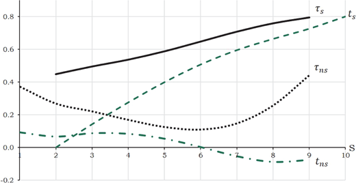
These results can be intuitively explained using Equations (34) to (38) that present firms’ choice variables as functions of the policy instruments. Figure 1 illustrates the two types of countries’ policy instruments as functions of the size of the coalition. First note that both types of countries set the tariff on foreign imports always higher than the tax on domestic production, the difference reflecting the fact that the tariff includes an environmental charge in addition to controlling import penetration into the domestic (or the coalition) market. For signatory countries, tariff and emission tax choices both increase monotonically with the size of the coalition. However, as the size of the coalition increases, t_s increases faster than τ_s, reflecting the need for controlling an increasing share of global emissions on which the tariff is zero.

On the contrary, nonsignatory countries choose an emission tax that is decreasing as the coalition grows, since on the one hand the environmental problem is increasingly taken care of by signatories and on the other hand, domestic production needs higher support since it is charged with a higher tariff in increasingly more foreign markets. Nonsignatories’ choice of tariff is decreasing up to some medium size of the coalition and then it increases. Since nonsignatories charge the same tariff to imports from all other countries, when the coalition is relatively small (the differential tariff treatment applies to small number of countries) nonsignatories decrease the tariff to improve trade among them. However, as the number of nonsignatories decrease, the incentive to protect local production from imports from signatories prevails and τ_ns increases at an increasing rate.

From equations (34) and (38), and Figure 1 it is clear that what drives exports from signatories to nonsignatories and prevents exports from nonsignatories to signatories when the coalition sizes are small, is that signatories choose a much higher tariff than emission tax. That is, members of a small coalition realize that a large share of global emissions originates from nonsignatories and thus choose a much higher tariff than tax, which promotes coalition members’ production and exports. As the coalition size increases, the difference between τ_s and t_s decreases, reducing signatories’ trade advantage. For larger coalition sizes nonsignatories provide a subsidy instead of taxing their domestic production, which allows them to export to signatories. It should be noted that if we restrict the tax level to positive values only, nonsignatories’ exports to signatories are zero.

Table 2 reports signatories and nonsignatories consumption and welfare levels, as well as total emissions and global welfare. It should be mentioned that in calculating total consumption for the cases that either one or both of $esnsX$ and $enssX$ become zero, we go back to the firms’ profit maximization problem given in Equations (32) to (33) and recalculate firms’ optimal choices in each situation. For example, for the case that $esnsX=enssX=0$⁠, firms’ optimal choices are, $esd(ts)=essX(ts)=ab−ts(s+1)b,ensd(tns,τns)=ab−tns+(n−s−1)τns(n−s+1)b$ and $ensnsX(tns,τns)=ab−tns−2τns(n−s+1)b$⁠, instead of those given in Equations (34) to (38). We also define firms’ optimal choices for the cases that either only $esnsX=0$ or only $enssX=0$⁠. At the third stage, firms know whether they will export to countries in the other group or not, so they can readjust their choices accordingly.

As was expected, total production and thus total emissions, presented in the second last column in Table 2, decrease as the size of the coalition increases.¹⁵Table 2 also presents welfare for signatories, W_s(s), and nonsignatories, W_ns(s), as well as global welfare, W_T = sW_s + (n − s)W_ns, as functions of the coalition size s.

Aggregate welfare increases with the size of the coalition. Apart from the very small coalition sizes, s = 2, 3, nonsignatories’ welfare always exceeds that of signatories, due to free-riding incentives, as is the case in environmental agreements that do not contain trade elements. It should be noted that in the absence of the environmental externality a trade agreement would yield continuously decreasing welfare to nonsignatories as the coalition increases (Yi, 1996).

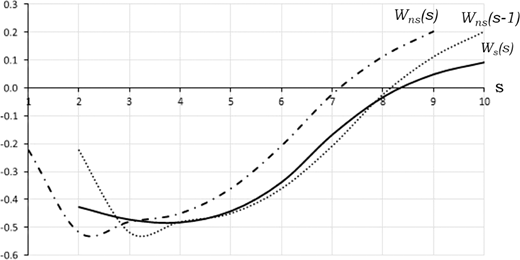
Figure 2 illustrates signatories’ welfare, W_s(s), by the solid curve, nonsignatories welfare, W_ns(s), by the dot-dashed curve and nonsignatories welfare sifted by one, W_ns(s − 1), by the dotted curve. The sifted welfare is added to the graph in order to assist in providing an illustration of the stability conditions graphically and allow us to specify the size of stable coalition(s).

The curves illustrating signatories and nonsignatories’ welfare have the same shape as those in the literature that examines environmental agreements without linkages to trade.¹⁶ However, there are some subtle but very important differences. The effect of linking environmental to trade issues is more prominent on the relative slope of the two curves, reflecting reduced free-riding incentives. In terms of Figure 2, the reduced free-riding incentives can be identified in that, for a range of coalition sizes, the welfare of nonsignatories does not increase as fast as that of signatories. This results in two intersections between the W_s(s) and W_ns(s − 1) curves, which as we explain in what follows is of great importance.

In order to determine the size of the stable coalition(s) we will refer to Figure 2. We start by noting that coalition s = 3 is internally stable, i.e., W_s(3) > W_ns(3 − 1), since the dotted curve is below the solid curve at s = 3. Moreover, s = 3 is externally stable, i.e., W_s(3 + 1) < W_ns(3) since the dotted and the solid curves intersect before s = 3+1. Therefore, the coalition of size s^* = 3 is stable. Note that, although the two curves intersect again between s = 4 and s = 5, coalition s = 4 is not stable because the W_ns curve intersects W_s from above and thus the stability conditions are violated. Furthermore, coalitions of size s = 5 and s = 6 are also not stable. At these coalitions the internal stability is satisfied, the external stability is violated and also the admissibility condition is violated as well since W_s(5) < W_s(6) and W_s(6) < W_s(7) respectively. Hence, coalition members become better off by expanding the coalition.

We now move to the coalition with seven members. This coalition is stable according to Definition 1 (i): none of its members has an incentive to withdraw (internal stability) and none of the outsiders has an incentive to join the coalition (external stability). In terms of Figure 2 observe that s = 7 is internally stable since the solid line is above the dotted line, i.e., W_s(7) > W_ns(7 − 1). Furthermore, s = 7 is externally stable, because W_ns(7) > W_s(7 + 1). Thus, the coalition of size s^* = 7 is stable.

Therefore, a joint trade and environmental agreement results in two stable coalition sizes: one small, which though is larger than the two-country agreement derived in the absence of trade, and a much larger one, which in the above example involves 70% of the total number of countries. Furthermore, this larger coalition yields substantial improvements in the global welfare. Using the values of global welfare W_T presented in the last column of Table 2, we can calculate the welfare improvements that each of the two stable coalitions provide relative to the smallest coalition (that is, W_T(3) − W_T(2) and W_T(7) − W_T(2)) as percentage of the maximum welfare improvement attained by the grand coalition (W_T(10)−W_T(2)). We find that while the small stable coalition attains only 3.87% of the potential welfare improvement, the large stable coalition yields a large share, 63.69%, of the welfare improvement that the grand coalition supports.

The following Remark summarizes the results of the above numerical analysis.

The results summarized in Remark 1 hold for all admissible values of the γ parameter. The larger stable coalition arises because the coalition members are able to counter the outsiders’ gains from free riding on their efforts to improve environmental conditions, by imposing a high tariff on their imports. As the coalition becomes larger, the benefits from free trade among coalition members increase and counterbalance the costs of environmental action. On the other hand the cost imposed on outsiders through the tariff increases as the coalition grows, since they are excluded from a continuously increasing market. Taking these costs and benefits into account, more countries have an incentive to join the coalition.

In this sub-section we examine the robustness of our main results, focusing on how they are affected when we change the number of countries, n. Since a affects only the vertical intercept of the demand function, see country i’s inverse demand function in Equation (4), setting a = 1 is a mere normalization. Furthermore, recall that we have combined, without any loss of generality, the two remaining parameters of the model, b and c, into $γ=cb$⁠. Setting b = 1, the value of c determines the value of γ. For any value of n we choose a value of γ, such that the positivity constraints for taxes, tariffs and emissions hold. Although, as in the case n = 10, we choose a value of γ close to the smallest admissible value, our results hold for all admissible values of the γ parameter.

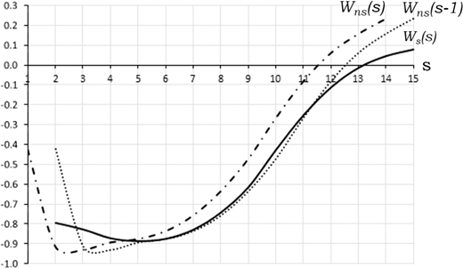
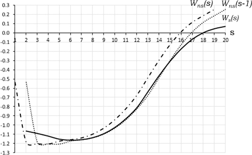
We start by presenting two indicative examples, n = 15 and n = 20 with the corresponding value of γ. In both cases, we use graphical analysis similar to the one in Figure 2. The solid curve W_s(s) illustrates the welfare for the signatories, the dot-dashed line W_ns(s) the welfare for the nonsignatories and the dotted line W_ns(s − 1) the welfare for the nonsignatories shifted by one.

In Example 1 we set n = 15, a = 1, b = 1 and γ = 0.025,¹⁷ and we illustrate the corresponding welfare curves in Figure 3. In order to control for the effect of allowing nonsignatories to provide subsidies to their firms, in this and the following example we impose a zero lower bound on nonsignatories’ emission tax. In this example, trade between signatories and nonsignatories takes place only for small coalitions, s = {2, 3, 4}, with signatories exporting to nonsignatories. For any larger coalition, i.e., s > 4, there is no trade between signatories and nonsignatories; trade is restricted among each group’s members.

This example also yields two stable coalition sizes. Although as n increases the distances between welfare curves become smaller, observe in Figure 3 that the W_ns(s − 1) curve intersects the W_s(s) curve from below in between s = 5 and s = 6. Therefore, the coalition of size s^* = 5 is stable since coalition s = 5 is internally stable, because W_s(5) > W_ns(5 − 1) and also externally stable, because W_s(5 + 1) < W_ns(5).

Furthermore, this example yields a larger stable coalition at s^* = 11. As illustrated in Figure 3, at s^* = 11, the solid line is above the dotted line, that is, W_s(11) > W_ns(11 − 1), guaranteeing internal stability and the solid line turns below the dotted line at s = 12, providing external stability to coalition of size 11, that is, W_ns(11) > W_s(11 + 1). In this example, the larger stable coalition involves 73.3% of the total number of countries. Furthermore, while the small coalition attains only 1.75% of the potential welfare improvement, the large one yields 70.71%, of the grand coalition’s welfare improvement.

In the second example we increase the number of countries to n = 20, we keep the same value for a = 1 and b = 1 and we define γ = 0.015.¹⁸Figure 4 illustrates signatories and nonsignatories’ welfare for these parameter values. Signatories export to nonsignatories for small coalition sizes, s = {2, 3, 4, 5}, while for larger coalitions trade is restricted among countries in the same group. Observe that in this example, the W_ns(s − 1) curve intersects the W_s(s) curve from below in two places, first between s = 6 and s = 7 and second between s = 14 and s = 15. Following the same process as in the previous two examples, we can prove that coalitions of size s^* = 6 and s^* = 14 are stable, since both internal and external stability conditions are satisfied. Similar to the previous two examples, the larger stable coalition consists of 70% of the total number of countries and attains 61.13% of the grand coalition’s welfare improvement, while the small coalition only 1.07%.

To further support the robustness of our results to changes in the model’s parameters, we increase the number of countries, choosing also admissible values of γ. Since the graphical presentation becomes less clear as the number of countries increase, we choose to present in Table 3 the main results for various values of {n, γ} up to n = 192, the number of member states in the UN. The first two columns present the choice of the model’s parameters {n, γ}. The third column presents the larger stable coalition size, max s^* and the fourth column this size as a percentage of n. The fifth column presents the welfare improvement the larger coalition achieves (∆W_T(s^*) = W_T(s^*)−W_T(2)), as a percentage of the maximum welfare improvement that the grand coalition can achieve (∆W_T(n) = W_T(n) − W_T(2)). Columns 6 to 8 present the respective data for the smaller stable coalition size denoted min s^*.

The data presented in Table 3 verify the robustness of our results to changes in the model’s parameters. We find that for any number of countries and the respective admissible values of γ, two stable coalition sizes emerge: a small and a large, with the latter involving consistently around 70% of the countries and achieving at least 58% of the potential gains from cooperation. These improvements from connecting a trade to an environmental agreement are due to the fact that the cost of staying outside of a trade agreement counterbalances the benefits of free riding on the environmental efforts of coalition members. The data in the last three columns show that even though the smaller stable coalition, attained at each {n, γ}, consists of 30 − 47% of the total number of countries, it achieves miniscule welfare improvements of no more than 7.5% of the potential. This smaller stable coalition is definitely larger that the two-country coalition we get in the absence of trade and resembles more the larger coalitions with low welfare improvements attained in Eichner and Pethig (2015) that allow for trade but do not use tariffs. Therefore, our analysis provides solid support for creating international agreements that determine jointly environmental and trade policies, since such agreements significantly increase the size of the coalition and provide strong environmental improvements that yield substantial welfare benefits.

This paper contributes to the literature by developing a model in which countries negotiate an agreement that defines a set of a tax on emissions and a tariff on imports. We build upon the strand of the literature specifying the formation of an international agreement as a non-cooperative game among countries. We extend the basic model by introducing a single firm in each country, all producing a homogeneous, polluting product which they can trade in a global market, assumed to be oligopolistic. Countries attempt to tackle the pollution problem and control trade by selecting the levels of an emissions tax and a tariff. Their choice of the level of these policy instruments could be unilateral or coordinated within a formal agreement. Signatories enjoy tariff-free trade among themselves, levy a tariff on imports from nonsignatories and an emission tax on their production. Nonsignatories levy a tariff on their imports and an emission tax on domestic production, taking into account only the effect of their emission on their own welfare.

This paper defines first the solution of two benchmark cases, reaffirming that the grand coalition yields lower global emissions and higher aggregate welfare than the Nash equilibrium. In defining the stable size of the coalition, we are able to derive analytical solutions of the above model only up to the second stage of the game. Thus, we resort to numerical simulations, which show that two stable coalition sizes emerge. The smaller stable coalition size although it can be substantial, including up to 48% of countries, it never provides substantial welfare improvements. The larger coalition size involves consistently around 70% of the countries and provides very substantial welfare improvements that are around 60% of the maximum welfare improvement provided by the grand coalition. A series of numerical simulations using different parameter values, three of which are diagrammatically illustrated in this paper, confirms that these results are robust to changes in the parameter values.

Although we are able to clearly demonstrate, using numerical examples, the effect that trade sanctions have on counterbalancing the free-riding incentives present in environmental negotiations, our results could be strengthened by deriving analytical solutions. This is one of the directions of future research, which also include allowing for different structures of the global market and determining endogenously a tariff among coalition members. It should also be noted that this paper’s modelling of trade is very abstract and does not take into account restrictions imposed by World Trade Organization (WTO). For example, WTO’s rule of non-discrimination principle, known as “most favoured nation treatment”, requires countries to grant equivalent treatment to the same products imported from any WTO member country.

Applying the assumption of symmetry across countries, allow us to write country i’s maximization problem (15) as,

Recall that, we define parameter γ as the ratio between environmental damages and benefits due to emissions, that is, $γ=cb$⁠. The reaction function for the equilibrium τ_nc (after imposing τ_nc = τ_i = τ_j and t_nc = t_i = t_j) is given by,

The reaction function for the equilibrium t_nc (after imposing τ_nc = τ_i = τ_j and t_nc = t_i = t_j) is given by,

The second-order condition for the signatories’ welfare maximization problem with respect to τ_s is satisfied,

The second-order condition for the signatories’ welfare maximization problem with respect to t_s is satisfied,

The second-order condition for the nonsignatories’ welfare maximization problem with respect to τ_ns is satisfied,

The second-order condition for the nonsignatories’ welfare maximization problem with respect to t_ns is satisfied,

The reaction function for the signatories’ equilibrium tariff τ_s(t_ns, τ_ns) is given by,

The reaction function is for the signatories’ equilibrium tax t_s(t_s, τ_s)

The reaction function is for the nonsignatories’ equilibrium tariff τ_ns(t_s, τ_s) is given by,