


Many sovereign wealth funds have expansive portfolios that give them the chance to influence markets through their investment choices. In this study, we analyze how oil extraction as a source of wealth influences portfolio allocation. We find that revenues from oil extraction affect the speculative motive and the hedging motives in opposite ways and create a portfolio allocation bias for oil-based funds. A numerical application of the model disentangles the motives and quantifies the bias. We find a positive bias in the portfolio allocation of an oil-based fund, which is increasing in the correlation of assets. Sensitivity analyzes show which parameters reduce the portfolio bias, turning the bias from "dirty" to "green" for large deviations from the default calibration. When a price on carbon is introduced, the intended reallocation of assets away from the oil-intensive sector is dampened by an amplification of the portfolio bias.
Introduction
Over the past three decades financial markets have witnessed the emergence of influential institutional investors known as the sovereign wealth funds (SWFs). SWFs manage state-owned stocks of wealth with the aim to maximize profits by investing in assets globally (Fotak et al., 2018). The majority of the top 20 SWFs derive their wealth from oil, whereby the extraction of mineral oil is their primary source of wealth. The oil-based funds of Norway and the United Arab Emirates are the largest SWFs in terms of assets under management (Fotak et al., 2018).
The rapid growth of SWFs in number as well as their assets under management have raised a number of concerns, two of which stand out: (1) Their sheer size endows SWFs with a market power, and (2) being state-owned creates the potential for strategic interests of the government to prevail over a pure profit maximization objective. Low transparency and lack of a liability structure complicates insight in the actual conduct of SWFs and thus add to these core concerns. This puts oil funds in a position where their investment strategy may affect market outcomes to their advantage. The literature on strategic behavior of SWFs has, to the best of our knowledge, not explored how the particular characteristics of SWFs (their size, as well as having an income stream connected to selling oil) can represent an incentive for SWFs to stimulate particular sectors of the economy. In this paper, we explore investment decisions of profit maximizing oil funds that are large enough to stimulate oil demand via their portfolio decisions.
The size of SWFs is at the root of the first concern. As of today, the top 100 SWFs manage approximately US trillion worth of assets (SWFI, 2023). SWFs control more than of all listed equities worldwide (Capapé and Santiso, 2017), and the 10 largest oil funds manage total assets between US$ 66 and US$ 825 billion - comparable to the annual GDP of many nations, safe the top 20 high income countries (Fotak et al., 2018; World-Bank, 2020). Given the size of their endowments, through their investment decisions, sovereign funds can potentially influence asset prices, the structure of the economy, and even the stability of the financial system as a whole. The investment of SWFs, for example when concentrated in small countries or specific sectors, could have a non-negligible effect on asset demand and drive up prices. The effect would be felt by other investors and would risk the creation of asset bubbles (Megginson and Fotak, 2015). In addition, the re-balancing of the large and concentrated investment positions of SWFs can be disruptive to financial markets. Shifts in the funds' asset allocations, or even just the perception of it, could lead to increased market volatility (Fotak et al., 2018). In the extreme, SWF may contribute to a destabilization of the financial system when their portfolio choices trigger herding behavior among other large financial actors (Lam and Rossi, 2010). This can be a double-edge sword, with SWFs creating momentum for more investments in small cap and emerging industries (like green technologies, for example), or furthering existing lock-ins in established technologies (like fossil fuel-based energy).
The second concern lies in the state-ownership of SWFs. While one of the main purposes of SWFs is to efficiently manage their endowments for current and future generations (Alan Gelb and Halland, 2014), governments may be tempted to advance less benign agendas by exerting their political influence on the fund's investment strategy, such as building political influence via stakes in the strategic infrastructure of foreign countries, or getting access to key technologies via the acquisition of innovative enterprises (Kamiński, 2017).
In general, however, empirical evidence suggests that SWFs tend to act as passive investors and in line with their stated objectives (Megginson and Fotak, 2015). Their scope and investment objectives can be grouped into three broad categories: capital maximization (savings funds), stabilization of the domestic economy, and economic development. The type and objectives of the SWF determine its investment behavior and horizon. For instance, capital maximizing funds tend to have a higher risk tolerance than stabilization funds and are likely to have a longer horizon. A stabilization fund has higher liquidity requirements, it will want to hold a higher share of its portfolio in liquid assets and will venture less in infrastructure projects that require long-term commitment. Portfolio diversification is particularly important for oil-based economies that rely on one main source of revenue, and therefore face volatility of public revenues due to the volatility of commodity prices. Oil-based SWFs therefore represent an opportunity for economies to ensure stable cash flow levels and provide funds for long-term investments. To this end, the optimal portfolio choice of oil funds would diversify away from oil-related assets, see for example Bremer et al. (2016) for an analysis of the specific hedging demand of oil-based SWF. Following this line of reasoning, one would expect oil-based SWFs to complement their portfolio by assets from renewable energy or other industries negatively correlated with the performance of the oil business.
Contrary to the diversification argument, there is empirical evidence for a bias toward their assets within the oil industry. For example, Chhaochharia and Laeven (2009) find that sovereign funds hold a disproportionately large fraction of their stocks in oil companies, and Bortolotti et al. (2015) cite SWF investment share in "oil and gas" at twice the level as their benchmark portfolio ( vs ). The underlying reasons may be behavioral, caused by a bias of investors to target sectors in their investment decisions that they are most familiar with (similar to the home bias, cf. Boyle et al., 2012; Coval and Moskowitz, 1999). As we will argue below, a dirty industry bias also follows from profit maximization when specifics of oil funds are taken into account in formal modeling. Raising market demand for fossil fuels through investments in dirty sectors of the economy can increase the profits from oil and thereby increase the wealth of the oil fund. Oil funds also have reason to be concerned about oil price dynamics: Fotak et al. (2018) point out the dramatic implication of a plummeting oil price for oil funds. In light of the upcoming ambitious climate policy measures these concerns can become particularly pressing (Ploeg, 2016).
A number of modeling studies have incorporated the defining characteristics of oil funds into the portfolio choice context. Scherer (2010) model the long-term perspective of SWF in a multi-period strategic asset allocation framework. Their analysis especially identifies the need for hedging against oil price shocks. Balding and Yao (2011) account for continuous depletion of oil resources in a dynamic portfolio model to find a superior asset allocation policy that is specifically tailored to oil dependent SWFs. Irarrazabal and Ma (2018) investigate, from a normative perspective, the optimal portfolio allocation between a risk-free and a risky asset of a commodity SWF with a long-term investment horizon. In their study, however, they abstract from any political and fiscal considerations. Bremer et al. (2016) argue that fund managers do not take into account oil price volatility and below-surface oil reserves in their investment strategies. Similarly, they argue that existing theories of optimal oil extraction do not take into consideration volatility of financial markets. Based on these postulates, the authors construct a theoretical framework unifying three streams of literature: portfolio choice theory, precautionary savings, and optimal oil extraction. According to Bremer et al. (2016) spending should be a share of total wealth, and precautionary savings should be adopted to manage any unhedgeable volatility. They also find that oil should be extracted faster than the Hotelling rule to generate a risk premium on oil wealth, in case oil prices are pro-cyclical.
Also with a focus on the rate of resource extraction, Marz and Pfeiffer (2023) present an equilibrium model where monopolistic resource extractors anticipate the effect of their extraction decision on oil demand and on a secondary income stream from investing oil revenues on the capital market. They determine when these new supply motives accelerate or postpone extraction, and resolve ambiguities in a numerical application of their model. In Marz and Pfeiffer (2020), they furthermore show that the resulting capital market effect works against the accelerating effect of a carbon tax on oil, thus dampening the "green paradox". These two papers explore fundamentally the same question as this study, namely the interaction of oil extraction and capital market but from a different perspective, namely the perspective of monopolistic resource extraction. By taking the perspective of a portfolio-optimizing investor, we focus on the investment problem of an SWF and include consideration of risk.
None of the studies on portfolio decisions of oil-based SWFs cited above consider the implications of their large size or the oil exposure of oil-based funds for their strategic behavior, for the emission intensity of the economy or for the effectiveness of climate policy in such settings (but see Way et al., 2019, which include anticipation of technological learning in portfolio decisions).
In this paper, we explore these aspects by looking at the differences in the investment behavior between a standard investor without connection to the oil industry and an oil-based fund that benefits from high oil demand via a revenue channel, but is also more exposed to risks related to the oil-intensive sectors of the economy via a risk-exposure channel. To quantify the effects of these channels, we calibrate the model parameters by using input-output data to adjust the parameters of the real economy, and returns and volatilities from exchange-traded funds (ETF) data for financial markets. The rest of the parameters are sourced from the literature. We calibrate the parameters according to three periods, where we notice a clear change in behavior of the green assets. We focus on the Post-COVID period as our default calibration.
Based on the calibrated parameter values, the oil fund's portfolio exhibits a bias toward the dirty sector. Varying the oil price reveals that differences in the portfolio are influenced by the oligopolistic price markup of oil extraction. While the standard investor's asset allocation is minimally affected by the oil price, the oil fund's investment in the dirty sectors increases with rising oil prices.
Robustness checks using alternative calibration periods confirm the persistent portfolio bias towards the dirty sector for the oil fund, with variations in asset returns and volatilities yielding proportional changes in the bias. The oil fund's portfolio bias is sensitive to risk aversion. Low risk aversion amplifies speculative demand, resulting in a bias towards dirty investment. As risk aversion increases, the bias shifts toward the clean sector. Relaxing assumptions about Leontief technology and correlation between clean and dirty assets, with higher elasticity of substitution, the bias diminishes.
The remainder of the paper is structured as follows. The next section introduces our model and analyses the portfolio allocation of an oil-based fund. In the section "Calibration", the model is calibrated. The section "Numerical Simulations" solves the model numerically to quantify the portfolio bias and investigate the effect of carbon pricing. The last section concludes the paper.
The Model
Our model links the portfolio allocation decision to a real economy with two sectors. The two sectors are modeled by representative firms that both employ capital to produce goods. In addition, the firm of the dirty sector uses oil as a second input factor while the green firm does not. The capital productivities are stochastic such that return on capital is risky with different expected return and volatility in the two sectors. This matters for investors, whose capital allocation to the sectors is determined by portfolio optimization. We contrast the allocation decisions of a standard portfolio optimizing investor with an oil-based fund that receives a share of oil extraction revenues in addition the portfolio return.
Firms
The representative firms of the green and dirty sector produce goods using a constant elasticity of substitution production technology. The index denotes green or dirty.
In Equation (1), is the share parameter that determines the importance of capital in production and is the elasticity of substitution. The factor productivities of capital and energy are random variables with a jointly normal distribution such that and are individually normally distributed with for and a correlation of .
For the remainder of this section, we focus on the case of perfectly complementary capital and energy ( ) to obtain closed form expression with an intuitive interpretation. The full model for arbitrary is solved in Appendix B and we include variations of in the numerical application of the model.
For perfectly complementary capital and energy, the production function takes the form of the Leontief technology. 1
In the dirty sector, the firm maximizes profit given the prices of the dirty good and fossil-fuel resource , and a carbon tax on fossil-fuel use such that profits are
The return on dirty capital thus becomes: 2
For simplicity, we assume that renewable energy only requires green capital . The return on green capital then becomes:
Equations (4) and (5) link expected sectoral returns to the underlying uncertainty about productivity.
where denotes profit per unit of effective capital .
The variances of the two returns are:
Standard Investor
In this section, we use the capital allocation decision of a standard investor as capital supply to the representative firms in the two sectors. The standard investor provides the benchmark for analyzing any distortions in the allocation decisions of an oil-based fund. For the purpose of our analysis, we assume a two-period scenario, where investors begin with a period 0 wealth of , which is then allocated to the two sectors to maximize utility, leading to the resulting period 1 wealth, . The period 1 wealth is given by:
where is the amount invested in the dirty sector and is the amount invested in the green sector. and are the returns on dirty and green assets, respectively. If we normalize the final wealth by current wealth we have:
Here, is the share of initial wealth invested in the green asset. We assume exponential utility, which we approximate by the mean-variance utility function over the normalized period 1 wealth:3
Here, is the expectation operator and is the variance operator. Bodnar et al. (2018) show that the coefficient of risk aversion in exponential utility can be linked to Value-at-Risk (VaR) considerations, which are commonly used by professional investors (VaR is, for example, the industry standard for risk management in financial institutions according to Ball and Fang (2006)). Using mean-variance utility therefore allows us to establish a link to industry practise while keeping the model tractable.
Using Equations (6) and (7), the expected normalized period 1 wealth is given by
The corresponding variance of the normalized period 1 wealth is given by
where maps correlation of capital productivities to correlation of returns.
The first-order condition maximizing over is:
We obtain the capital allocation of the representative investor by solving the above first-order condition for the green capital allocation :
and since , the dirty capital capital share is:
The above solutions are the standard portfolio allocations for a mean-variance utility function with two risky assets (see, for example, Tobin et al., 1965). Equations (18) and (19) follow the convention of separating the demand for green and dirty assets into the speculative demand and hedging demand (the two large fractions), where the speculative demand is mainly driven by the excess return of one asset over the other, with decreasing relevance in the risk aversion (cf. Ghosh, 2010). The hedging demand is driven by the relative volatility of the other asset (notice that the denominator is the total portfolio variance, and the hedging demands of the two assets add to 1 and, therefore, are complementary), such that risk is hedged by shifting the portfolio the other way. It is decreasing with a positive correlation and disappears for perfect correlation and same volatility of the two assets.
Since we have assumed a linear technology for final good production, in equilibrium the returns are determined by the energy supply side alone and we can simply insert the expressions for the expected returns as determined by the energy supply part of the model given by Equations (6) and (7) as well as the variance expressions (8) and (9), to determine the equilibrium capital shares:
where is the profit per unit of effective capital ( ), and P converts correlation of returns into correlation of factor productivities (as defined for Equations (6) and (16), respectively).
The excess return in Equation (21) is increasing in the price of dirty output , and decreasing in the oil price and the carbon . The reason is straight forward: both increase the cost of dirty production and, therefore, reduce the return on capital. A positive correlation of the dirty and green assets will reduce the importance of the hedging demand relative to the speculative demand, intuitively by making the two assets more alike. 4 Conversely, negative correlation raises the hedging demand for the other asset, as anti-correlated assets create additional possibilities to diversify risk.
Oil-based Fund
The oil-based fund invests in the same asset universe as the representative investor but benefits from an additional source of income as compared to conventional investors - namely revenue from oil extraction. We assume that oil extraction is operated by a separate entity, which is a common division of responsibilities in states that have oil-based funds.5 To account for the large size of oil-based funds, we
include the effect of investment on oil demand, such that an incentive emerges to strategically invest in oil-intensive industries to increase income from oil extraction.
For Leontief production technology, it is possible to express as:
We assume imperfect competition in oil extraction such that the oil price exceeds marginal costs . Specifically, we assume oligopolistic competition such that the price markup can be expressed by with (see Appendix A for a derivation). The oil fund takes as given when deciding on investments. This results in the following specification for oil business profits and the return on capital for the dirty sector:
The oil demand stemming from the investment activity of the rest of the economy is and is taken as given by the fund. As the oil fund can only control the oil demand that results from its investments , we distinguish it from the investment of others in the dirty sector, . The normalized period 1 wealth of the oil fund reads:
where and represent the fractions invested in both sectors, is the relative size of the fund to the rest of the economy in terms of wealth, and is the relative weight of investment in the dirty sector for the rest of the economy, i.e., . Hence, the first term in Equation (24) represents the profits from the oil business, while the second and third are related to the investment income.
After inserting the specifications for and from Equations (4) and (5) we get:
After rearranging, we obtain:
Defining , the expected value of the normalized period 1 wealth of the oil fund reads:
The variance of the normalized period 1 wealth of the oil fund is:
Notice that when compared to the variance of the wealth of the standard investor (16), the oil fund is more exposed to the dirty sector risk when reallocating capital (changing ) since . This can be explained by the fact that reallocating capital toward the dirty sector increases oil demand and increases the potential impact of shocks on profits, since a greater share of the profits are dependent on oil. We can now insert Equations (26) and (27) into Equation (12) and maximize over . This implies the following first-order conditions:
Solving for yields:
and
where
and
Differences in Asset Allocation
The differences between the capital allocation of the oil fund and the capital allocation of the representative investor is in the additional expression , which is the oligopolistic markup of resource extraction per unit of oil, converted to units of output by the oil efficiency , and therefore captures the additional income that accrues to the oil fund. We identify three channels through which the oil extraction markup affects the portfolio of the oil fund but not the standard investor.
Revenue Channel
First, the oligopolistic markup has a positive effect on the excess return of the dirty assets over the green asset for the oil fund (the numerator of the speculative demand), see Equation (29) compared to Equation (21).
Therefore, as long as the oil price exceeds extraction costs and all else equal, the speculative demand for dirty assets is increasing in the markup on oil extraction, which shifts the portfolio toward more investment in the dirty asset.
Portfolio Risk Channel
Second, the markup also affects the denominator of the speculative demand, which is the total variance of the portfolio. For , the total portfolio variance is larger the oil-based fund. The higher portfolio variance works like a risk adjustment of the excess return, making the oil-based fund less sensitive to higher returns. Intuitively, for the oil fund, oil demand risk adds to the dirty sector risk. All else equal, this channel will reduce the portfolio allocation of the oil-based fund to the dirty sector.
Risk Exposure Channel
Third, the higher level of risk of the dirty asset for the oil-based fund also affects the oil fund's hedging demand. Formally, the volatility of dirty assets is larger for the oil fund, , again, when . The increased risk associated with dirty assets increases the hedging demand for green assets in Equation (28) and, by increasing the weight , shifts the portfolio away from dirty assets.
In equilibrium, the total effect of the three channels is ambiguous because the revenue channel moves the portfolio allocation in the opposite direction of the portfolio risk channel and the risk exposure channel. A non-zero correlation will also affect the relative strength of the channels. A positive correlation reduces the value of either of the two assets for hedging risks, it therefore enters negatively in the hedging demand. As the oligopolistic markup increases the volatility of the dirty asset ( in ), this effect of correlated asset returns also has a stronger effect on the hedging demand in of the oil fund. The portfolio variance (the denominator) is reduced for correlated assets. As this affects the two terms in Equations (28) and (29) equally, it does not affect the balance of the speculative and the hedging motives. Still, whether the portfolio decisions is ultimately biased toward a specific sector in our economy thus becomes a numerical question. The relative strength of the channels will depend on the magnitude of the markup relative to , which for fixed extraction costs is determined by the oil price , and by the relative importance of speculative demand and hedging demand, determined by the risk aversion . To determine the direction and magnitude of the overall effect, we provide a numerical simulation of the model in the next sections.
Calibration
We rely on input-output data to calibrate the parameters of the real economy, and ETF data for financial returns and volatilities. Other parameters are taken from the literature as detailed below.
Sector Definition
We divide the real economy as well as the asset universe into two sectors: A dirty sector that relies on oil as an input to production, and a clean sector, which is the rest of the economy. We use input-output data for the U.S. economy from the WIOD project (Timmer et al., 2015, 2015 release) complemented by energy data from Corsatea et al. (2019) to identify the industries with the largest demand for oil. Sectors are weighted by their size, which we proxy with capital stocks from complementary socio-economic accounts (Gouma et al., 2018). We find that largest demand for oil arises from (i) transport by air, water, and land, (ii) the chemical industry, and (iii) construction. Table 1 reports the demand shares as well as the relative weight of the industries within the dirty sector. Together, the selected sectors account for almost half of total oil use ( ) but just of economic output.
Returns and Volatilities
Expected (nominal) returns and volatilities for the green and dirty sectors are derived from ETF prices that include broadly the same
Dirty sectors.
| Sector | NACE | Oil demand share (%) | Weight |
|---|---|---|---|
| Transport (land, water, air) | H49, H50, H51 | 28.62 | 0.54 |
| Manufacture of chemicals and chemical products | C20 | 11.99 | 0.32 |
| Construction | F | 8.31 | 0.14 |
| Total | 48.92 | 1.0 |
Oil demand is the sectors demand relative to total oil demand. The relative weight is capital of the industry relative to capital of the selected "oil-intensive" industries. Sectors are classified using the Statistical Classification of Economic Activities in the European Community (NACE). economic activities as the industries in Table 1. We use the iShares U.S. Transportation ETF (ticker symbol IYT), Basic Materials ETF (IYM), and Home Construction (ITB) as a proxies for the returns from investment in transport, chemicals, and construction. For these three ETFs to jointly represent the dirty sector, we consider a portfolio where each ETF is weighted by its size given by the relative share of the industries' capital (the weights are given in Table 1). Adjusted share prices were obtained from Yahoo Finance; portfolio return and volatility were calculated following standard equations (e.g., Berk and DeMarzo, 2013, Equations (11.3) and (11.11)).
Table 2 shows the resulting expected returns and standard deviations . We exclude the time of the global financial crisis of 2008 and the SARS-Cov2 pandemic, as well as the 2014-2015 oil price decline due to its exceptional impact on oil price and the dirty portfolio, and estimate returns and volatilities separately for the relatively stable times in-between (cf. time series of prices in Figure 1). We use the most recent period (Post-COVID) as our benchmark but explore the Pre-Decline and Pre-COVID Scenarios to test the robustness of our
Sector returns and volatilities.
| Scenario | ||||
|---|---|---|---|---|
| Parameter | Pre-Decline | Pre-COVID | Post-COVID | |
| Green | Return | 0.180 | 0.157 | 0.305 |
| Volatility | 0.169 | 0.128 | 0.165 | |
| Price | 0.366 | 0.319 | 0.620 | |
| Volatility | 0.462 | 0.401 | 0.267 | |
| Return | 0.186 | 0.142 | 0.375 | |
| Dirty | Volatility | 0.223 | 0.161 | 0.211 |
| Price | 0.218 | 0.155 | 0.346 | |
| Volatility | 1.483 | 1.407 | 0.700 | |
| Correlation | 0.922 | 0.855 | 0.813 |
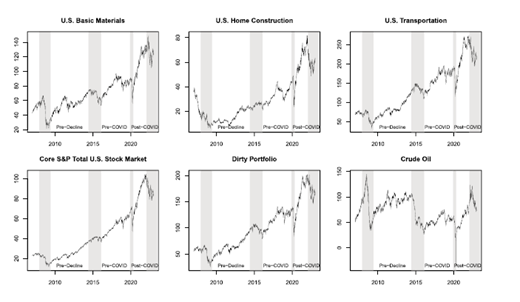
results (see Appendix C). In the default calibration, the dirty sector exhibits a higher return but also a higher volatility.
The green sector is the complement of the dirty sector. We derive returns for the green sector by factoring out the dirty sector returns from the market portfolio, represented the iShares Core S&P Total U.S. Stock Market ETF (ITOT), an ETF that tracks the total market. As above, we use the relative size of capital stocks as portfolio weights.
Table 2 includes the coefficient of correlation of the dirty and green returns (from the time series of ITOT returns and the dirty portfolio returns), which is approximately 0.9 in all time periods considered. The high positive correlation is plausible, since the selected dirty industries are procyclical (high beta) industries. We view this value as an upper bound since the overlapping definition of dirty and green sectors may exaggerate the correlation.
Technology Parameters
The efficiency parameters of capital use in production ( and ) and oil-use ( and ) are calibrated using output, capital, and oil-use data from WIOD and the associated socio-economic accounts (Table 3) and exploiting that for Leontief production, . The output prices and are chosen to align the stochastic efficiency parameters and with the sector returns and according to Equations (6) and (7). The corresponding volatilities and follow from Equations (8) and (9).
For the elasticity of substitution between factor inputs to production, our benchmark is the case of Leontief technology with perfect complementarity of capital and oil-use, i.e., in Equation (1), but we explore in parameter variations. Strong complementarity of capital and energy is indeed supported by empirical evidence as well as common practice in modeling. For example, Zha and Zhou (2014) consider different nesting structures for capital, labor and energy in production functions with constant elasticity of substitution. For the elasticity of substitution between energy and a capital-labor composite Zha and Zhou (2014, Table 4) cite five values well below unity for :
, and (the latter three times). Since we consider only capital and energy (oil) but no labor, our technological assumption is closest to this setting. We explore the value as an alternative to the Leontief assumption (i.e., ).
Preference Parameter
For the coefficient of absolute risk aversion , modeling studies commonly use values ranging from 1 to 10 (Bodnar et al., 2018). Examples where models with absolute risk aversion are calibrated for exemplary or illustrative numerical application are Wills (2018, ), Yang and Li (2013, ), Baker et al. (2022, ), and Kelsall et al. (2023, ).
The broad range of values in model calibrations is mirrored by empirical studies. Summarizing empirical studies that estimate risk aversion based on household consumption data, Bucciol and Miniaci (2011) report a range of 2-7 for studies based on pseudo-panels, and values "well above 10 " for studies based on macroeconomic statistics. In their own analysis of household portfolios, they calculate average risk aversion based on mean-variance portfolios of financial assets ( ), and portfolios that include human capital and real-estate ( , and when applying constraints such as "no short-selling").
Bodnar et al. (2018) show that the optimal mean-variance portfolio can be linked to a minimum value-at-risk portfolio, which is relevant for investors that are bound to value-at-risk considerations by regulation of the financial sector. Whether value-at-risk regulation, which frequently covers financial institutions like banks, extends to oil funds, is not clear (e.g., not disclosed by oil funds). The study computes the implied risk aversions for minimum value-at-risk portfolios at the "commonly used" confidence level of . The resulting coefficients of risk aversion fall within the range [15, 45] (see Fig. 2, upper left panel in Bodnar et al., 2018, p. 312).
We select as a value at the center of the [1,10] range supported both by empirical research and modeling practice, and that is close to Bucciol and Miniaci's (2011) estimate for the "financial portfolio" ( ), which is closest to the investment decision in our model. To reflect the broad range and large uncertainty we consider a range of that includes the lower bound of the high estimates from Bodnar et al. (2018).
Oil Extraction
Oil extraction is characterized by the oil price and the marginal extraction cost of oil . We set the oil price to the average price of near-term Crude Oil futures (ticker symbol CL ) for the same time period as the ETF prices (Table 4).
The marginal extraction costs vary strongly depending on the type of crude oil and the site location. Masnadi et al. (2021) report a range of to for crude type and a range of to for the top 30 global producers of crude oil. To select a value from these ranges, we follow Genc (2017) who quotes a medium value of for OPEC from Reuters with and as low and high values, which falls well within ranges of Masnadi et al. (2021).
For the market power on the oil market, our choice of oil price and marginal extraction cost implies a Lerner index of LI 0.80 (for comparison, Genc (2017) reports a range of [0.71, 0.90]). For the corresponding oligopolistic price markup we have .
To convert $/bbl to tril$/EJ, we assume an energy intensity of 42GJ per tonne of oil, approx. 7 bbl , therefore approx. , or a factor of (Wikipedia, 2023) to go from to . To convert Giga to Exa and dollars to trillion dollars is a factor of 0.001 . Thus, we convert from to tril$/EJ by multiplying with 0.000167 .
Numerical Simulations
In our numerical simulations, we start with the calibration of the basic model with Leontief technology, no asset correlation and no climate policy , then we explore the implication of relaxing these assumptions.
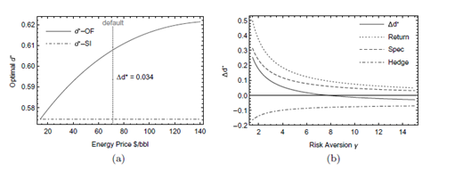
Asset allocation . The left panel shows the optimal allocation to dirty assets for standard investor (SI) and oil fund investor (OF). The difference in in the right panel is also shown for an investors who only considers the excess return (Return) or speculative demand of oil funds (Spec), or only considers their hedging demand (Hedge).
Asset allocation . The left panel shows the optimal allocation to dirty assets for standard investor (SI) and oil fund investor (OF). The difference in in the right panel is also shown for an investors who only considers the excess return (Return) or speculative demand of oil funds (Spec), or only considers their hedging demand (Hedge).
Portfolio Bias
We find that in our default calibration, the portfolio allocation of the oil fund is biased toward investment in the dirty sector. Figure 2 shows the asset allocation weight in equilibrium for the standard investor and the oil-based fund. We vary the energy price (oil price) as we know from Equations (21) and (29) that differences in the portfolio will be driven by the oligopolistic price markup of oil extraction. While the effect of the oil price on the asset allocation of the standard investor is negligible, the investment in the dirty sectors by the oil fund is increasing in the oil price. We know from Equations (21) and (29) that of the oil fund - in contrast to of the standard investor - is affected by the oligopolistic price markup. Figure 2A shows that the positive price markup of an oil price above extraction cost creates a portfolio bias toward the dirty sector for the oil fund, with the bias rising to 4.7pp (percentage points) for an oil price of . We test the robustness of this result by calibrating the model for asset returns and volatilities from the alternative time periods reported in Table 2. Appendix C has the corresponding figures. The results are qualitatively the same and quantitatively similar. When the data suggests lower excess return of the dirty asset and higher volatility, we see a smaller portfolio bias towards the dirty sector.
The portfolio bias of the oil-based fund is sensitive to the degree of risk aversion of the investor. Figure 2 B shows how the bias as the difference of portfolio weight of oil-based fund minus standard investor's portfolio weight . In addition to the oil fund's bias toward the dirty sector , we show the bias for an investor taking only the revenue channel (i.e., the effect on excess return, dotted) into account, an investor taking revenue channel and portfolio risk channel into account (i.e., the "risk adjusted excess return" that creates speculative demand, dashed), and an investor taking only the risk-exposure channel into account (i.e., the effect on the hedging demand, dot-dash). As discussed in the section "Differences in Asset Allocation", the revenue channel implies a higher speculative demand for the oil-based fund, whereas the risk-exposure channel reduces its hedging demand, and consequently the higher excess return ("Return") and - to a lesser extend - the higher speculative demand ("Spec") create a bias toward the dirty asset. In contrast the reduced risk exposure decreases the hedging demand ("Hedge"), which by itself biases the oil-based fund toward green sector investment.
Low risk aversion puts the emphasis on the speculative demand bringing the total effect close to the dashed line. At , the bias is 17 pp . With increasing risk aversion more weight is put on the hedging motive, around the two effects cancel out, at still higher levels of risk aversion, the oil fund is biased toward the clean sector. The risk aversion of the investor is therefore decisive for the portfolio allocation bias. If fund managers act with a risk aversion comparable to the investors in household portfolio studies, the weight on the speculative motive is enough to create a bias towards dirty investment. Higher degrees of risk aversion can be interpreted as fund managers that follow value-at-risk considerations at high confidence levels. The resulting high preference for diversification creates a bias toward green assets to hedge the income from oil extraction.
Next, we explore the effect of relaxing the assumptions of Leontief technology and no correlation on the portfolio bias of the oil-based fund
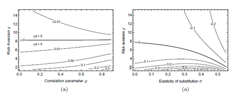
Allocation bias of oil funds. At the locus in the contour plots, the portfolio bias of the oil fund flips from "dirty" ( ) to "cleaner" ( ).
Allocation bias of oil funds. At the locus in the contour plots, the portfolio bias of the oil fund flips from "dirty" ( ) to "cleaner" ( ).
in Figure 3. Figure 3A shows that for risk aversion below , the bias is increasing in the correlation of clean and dirty assets. The effect is strongest for low . At , the bias increases from less then 10 pp to more than 30 pp . At our default risk aversion of the effect is less pronounced: increases from below 1 pp to about 5 pp .
The effect of the elasticity of substitution on the portfolio bias is shown in Figure 3B. When capital and energy (oil) are perfect complements, the demand for oil from the dirty sector and revenues from extraction for the oil-based fund rise in proportion with the additional investment in the dirty sector. When the elasticity increases, substitution of capital for oil in the dirty sector dampens the additional demand for oil and subsequently the additional revenues of the oil-based fund. Consequently, the area with in Figure 3B shrinks with an increasing elasticity. For and our alternative calibration value of the portfolio bias has all but vanished.
Finally, we explore an extension of the asset universe by including the option to invest in a risk-free asset (see Appendix B.3). We find that in principle, our analysis carries over to this three-asset model, and as in the two-asset case, a portfolio allocation bias of the oil-based fund emerges that is driven toward dirty investment by an excess return motive, and driven toward green investment by an increased risk of the dirty asset. The main differences are, first, that risk aversion has a less prominent role: it is decisive for investment in the riskfree asset but does not affect the portfolio bias. Second, the portfolio allocation becomes more sensitive to asset volatility, as it takes the place of total portfolio volatility in the speculative demand. With the returns and volatilties that we estimate, avoiding the additional risk from the extraction revenues outweighs the additional return such that the portfolio of oil-based fund is biased toward green investment. Thus, although the mechanisms of the portfolio bias are robust under this variation of the asset universe, this extension showed that alternative assumptions about the portfolio choice problem of the fund manager can have a substantial impact on the relative importance of the channels of the bias.
Climate Policy
For investors who are guided by a mean-variance utility, the impact of a carbon tax on the allocation of capital to dirty assets is not analytically straightforward. An increase in the carbon tax reduces the dirty sector's profit but also reduces the volatility of returns of that sector. The figures below the effect of the carbon tax on dirty assets allocations. Figure 4 shows the effect of a carbon tax up to
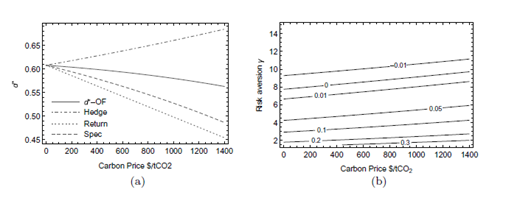
Climate policy implications on the optimal allocation to the dirty sector (left) and on the portfolio bias of the oil fund toward the dirty sector (right).
Climate policy implications on the optimal allocation to the dirty sector (left) and on the portfolio bias of the oil fund toward the dirty sector (right).
Figure 4A shows the optimal allocation to the dirty sector. For the oil fund investor, is declining in the carbon tax. Again, we decompose the effect of the carbon tax on the portfolio along the impact channels by showing portfolio allocation of investors where the carbon tax affects only their excess return ("Return"), or their speculative and hedging demands ("Spec" and "Hedge", respectively). The carbon tax reduces the return on dirty assets, hence lowering their excess return over the green asset and, therefore, reducing the demand for dirty assets (dotted line). At the same time, lower returns imply a lower volatility. The "risk-adjusted" return in the speculative demand therefore falls less rapidly, and the hedging demand is increasing in the carbon tax because less green assets are needed to hedge the (decreased) risk of the dirty asset (dash-dot line).
The effect of the carbon price on the portfolio bias is shown in Figure 4B. The bias of the oil-based fund toward dirty assets for risk aversion below remains under carbon pricing. In fact, carbon pricing reinforces the bias: at a given degree of risk aversion , the bias increases, and with higher carbon prices, the portfolio is bias towards the dirty sector for higher degrees of risk aversion (up to ). Intuitively, carbon pricing affects emissions from oil use but not revenues from oil extraction, and therefore has an impact on return on capital but not on the oligopolistic price markup, see Equation (29). The importance of the price markup is therefore increasing in the carbon tax; and consequently the portfolio bias is increasing in carbon tax.
Conclusion
In this study, we take first steps to include the motivations and strategic options available to large oil funds in a formal analysis of their investment and portfolio decisions. Specifically, we extend the portfolio allocation problem of an oil-based fund by modeling a demand stimulating effect of additional investment in oil-intensive sectors of the economy and including revenues from oil extraction as part of the fund's wealth.
We find that including oil extraction revenues affects the portfolio allocation to the "dirty" sector through three channels. First, oil extraction revenues increase the excess return of investment in the dirty sector, increasing the oil fund's speculative demand, such that the oil fund's portfolio is biased toward dirty assets. Second, larger returns also increase the volatility of the dirty asset and hence the total portfolio variance, which acts as a "risk-adjustment" of the speculative demand, shifting the asset allocation away from dirty assets. Third, the increased volatility also affects the hedging demand: the demand for green assets rises to hedge the increased risk of dirty assets. This shifts the portfolio toward green assets and away from dirty assets.
The numerical simulations of the model help to disentangle the ambiguous overall effect on asset allocation. We find a substantial portfolio bias of the oil-based fund toward investment in sectors with a high demand for oil in our default calibration. The result is robust for alternative calibrations and for broad ranges of parameter variations. However, the portfolio bias decreases and vanishes for high elasticities of substitution of capital for oil and high degrees of risk aversion. Since we cannot precisely pin down the risk aversion oil-fund managers, some uncertainty remains regarding the sign and magnitude of a potential portfolio bias.
When carbon pricing reduces the return on capital from the oilintensive sector, the divestment from dirty assets is slowed down because a reduced risk of dirty assets, also due to carbon pricing, provides a motive to hold more dirty assets. As this effect is stronger for oil-based funds, carbon pricing reinforces the portfolio allocation bias. This portfolio bias, however, is small compared to the divestment.
Appendix
A. Oligopolistic Oil Extraction
It is well known in industrial organization that oligopolistic firms will sell their goods at a price above marginal cost (e.g., Francois and RolandHolst, 1997). In this appendix, we apply standard arguments to show that oligopolistic oil extraction implies a resource price of
where is the number of extraction firms, is the price elasticity of demand for oil, and is the market response to a change in supply by firm , as expected by firm . For and finite is typically greater than unity.
To see that Equation (30) holds, assume an oligopoly of oil ( ) extracting firms with profits for the individual extracting firm:
Each firm's behavior is determined by the first-order condition of optimality
with the elasticity of demand for oil and the the expected market response to changes in oil supply by firm we have:
and for symmetric extracting firms with equal market share we have
where the left-hand side is known as the mark-up ratio. The price as in Equation (30) follows.
B. Generalized Model
With the CES production function, the firm's profit can be expressed as:
The return on dirty capital thus becomes:
Since we assumed that renewable energy only requires green capital . The return on green capital remains the same as in the special Leontief case:
The expected returns are given by:
and
The expected return on dirty capital is positive, i.e., . The variances of the two returns are:
and
Standard Investor
The period 1 wealth is given by:
where is the amount invested in the dirty sector and is the amount invested in the green sector. and are the returns on dirty and green assets, respectively. Normalizing the final wealth by current wealth we have:
Here, is the share of initial wealth invested in the green asset. Both investors have exponential utility, which we approximate by the meanvariance utility function over the normalized period 1 wealth:
where is the expectation operator and is the variance operator.
The expected normalized period 1 wealth is given by:
where and are given by the energy supply side that was developed in the last section. After inserting the specification derived from the energy supply part of our model (i.e., Equations (34) and (35)) we get:
The variance of the normalized period 1 wealth is given by:
or after inserting the specification derived from the energy supply part of our model:
Where
.
The first-order condition maximizing over is:
We obtain the capital allocation of the representative investor by solving the above first-order condition for the green capital allocation :
and since , the dirty capital capital share is:
Inserting the expressions for the expected returns as determined by the energy supply part of the model given by Equations (34) and (35), as well as the variance expressions (36) and (37), to determine the equilibrium capital shares:
where
and
Oil-based Fund
For CES technology, it is possible to express as:
For simplicity, we assume a constant marginal extraction cost and no fixed extraction cost, which results in the following oil business profit specification:
The normalized period 1 wealth of the oil fund reads:
After inserting the specifications for and from the energy supply part of the model we get:
where
After rearranging, we obtain:
Defining , the expected value of the normalized period 1 wealth of the oil fund reads:
The variance of the normalized period 1 wealth of the oil fund is:
Inserting Equations (50) and (27) into Equation (12) and maximize over . This implies the following first-order condition
Solving for yields:
and
where again
and
The "speculative" demand for the dirty asset, which we define simply as the difference in the returns associated with the dirty and green assets (see Equation (53)):
The "diversification motive", which we define simply as the first term in Equation (29):
The Portfolio with Risk-free Asset
When we include a risk-free asset, the wealth becomes
As for the oil fund's normalized period 1 wealth, we have:
where again
and
The investors' mean-variance utility for :
The expected portfolio return is given by:
Similarly, the expected portfolio return for the oil-fund is given by:
where is as defined above.
The variance of the portfolio return as in the prior case is given by:
Similarly, the variance of the portfolio return for the oil-fund is given by:
We take the partial derivatives with respect to and in both cases and set them equal to zero , to obtain the optimal weights and :
The first-order conditions for optimality are:
Solving these equations simultaneously to find and . The solutions for the standard investor are:
where as defined above
The solutions for the oil-fund are:
Equation (67) shows that for the three-asset model has only a speculative demand (first term in the bracket) but no hedging demand. Instead, an investor with a higher risk aversion will reduce their holding of both risky assets and, consequently, increase the share ( ) of the risk-free asset.
For the oil-based fund, , and hence their speculative demand will be higher than the standard investors due to the higher excess return in the numerator - but also lower than the standard investors due to the larger asset variance in the denominator. Whether the effect on excess return or the effect on asset volatility dominate implying a higher or lower speculative demand depends on the relative size of mean and variance of the productivity.
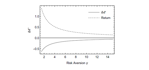
Figure 5 shows the difference in allocation of the dirty sector between the oil fund and the standard investor for our default calibration. The model shows a great sensitivity: at a low risk aversion, the portfolio allocation would be biased toward dirty investment by 100 pp . If the excess return is risk-adjusted such that the full speculative demand is taken in to account, the bias flips to green investment, with a portfolio allocation bias of -50 pp .
Figure 5: Portfolio allocation bias for two risky and a risk-free assets. The figure shows difference in the allocation to the dirty sector by the oil-based fund for the Post-COVID Scenario as defined in Table 2.
Portfolio allocation bias for two risky and a risk-free assets. The figure shows difference in the allocation to the dirty sector by the oil-based fund for the Post-COVID Scenario as defined in Table 2.
Portfolio allocation bias for two risky and a risk-free assets. The figure shows difference in the allocation to the dirty sector by the oil-based fund for the Post-COVID Scenario as defined in Table 2.
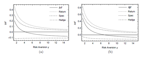
Portfolio allocation bias for alternative calibration scenarios. The panels show difference in the allocation to the dirty sector by the oil-based fund for the Pre-Decline Scenario (left) and the Pre-COVID Scenario as defined in Table 2.
Portfolio allocation bias for alternative calibration scenarios. The panels show difference in the allocation to the dirty sector by the oil-based fund for the Pre-Decline Scenario (left) and the Pre-COVID Scenario as defined in Table 2.
C. Alternative Calibration Scenarios
Figure 6 shows the portfolio allocation bias of the oil-based fund for the alternative calibrations to the time from June 2009 to June 2014 (Pre-Decline Scenario, left panel) and from February 2016 to December 2019 (Pre-COVID Scenario, right panel) as defined in Table 2. The figures are qualitatively the same as Figure 2.
In the Pre-Decline Scenario has a lower excess return of the dirty asset over the green asset and than the default (Post-COVID) scenario and a higher volatility. This reduces the "Return" and "Spec" motives and strengthens the "Hedge" motive. We still observe a substantial portfolio bias toward dirty assets but the bias flips from dirty to green at a lower risk aversion of about .
The Pre-COVID Scenario falls in-between the other two scenarios in terms of volatility but exhibits a lower expected return for the dirty compared to the green asset. This puts the Pre-COVID Scenario inbetween the default and the Pre-Decline Scenario.
Acknowledgment
We thank Beatriz Gaitan for economic modeling advise in the model extensions, and participants in the Research Seminar of FutureLab PECF at PIK for feedback and helpful comments. This research was supported by the German Federal Ministry of Education and Research (BMBF) [grant no. 01LN1703A and 01LA1824A], which we gratefully acknowledge.
References
Note that while the share parameter is lost for , the factor productivities are preserved.
This amounts to an equilibrium condition, equilibrating the energy supply side with capital supply side. Under this condition, if final good production is not linear in and , the actual return would also be determined by the capital supply side (i.e., would be a function of and ), but for a linear production function the marginal product is always constant ( is a parameter).
Maximizing exponential utility is equivalent to meanvariance maximization when is normally distributed, i.e., we implicitly assume that our returns have approximately a normal distribution. Mean-variance utility has also been shown to be a good approximation for a wide range of utility functions (Levy and Markowitz, 1979).
The correlation P affects the denominators of hedging demand and speculative demand in the same way, such that the denominator does not affect the relative contributions of hedging demand and speculative demand.
For example, in Norway, the United Arab Emirates or Saudi Arabia, oil extraction is operated by state-owned corporations (by Equinor, the Abu Dhabi National Oil Company and Saudi Aramco, respectively), while investment and asset management of (part of) their revenues is delegated to funds (to the Government Pension Fund Global, the Abu Dhabi Investment Authority and the Public Investment Fund, respectively).
We separate our consideration of acting strategically on capital markets (to affect oil demand) from imperfect competition on markets for oil due to monopolistic market power of oil suppliers. See Marz and Pfeiffer for an analysis where monopolistic market power in extraction is taken into account.
Ideally, the ETFs would form an efficient portfolio of their assets. By using the relative capital shares, we approximate their weights in the market portfolio, which is efficient. Moreover, the relative capital share is an indicator of investment opportunities and the ability of the industry to absorb additional investment, therefore we avoid the less plausible case of focusing investment on an industry with a relatively small capital stock.
Technically, we use the ITOT ETF to find the market returns at time . Assuming that is the portfolio return of the green and dirty returns (with shares ), we can calculate the green return as .
When we explored in our model numerically we found no substantial differences from , as the hedging demand is already the dominant incentive at such a high risk aversion (e.g., the portfolio bias in Figure 2B is almost flat at ).
For "Return", we eliminate the additional terms of the oil fund (the oligopolistic price markup) everywhere in (29) except in the excess return, i.e., the numerator of the speculative demand. For "Spec", we eliminate the oligopolistic price markup from the hedging demand. Finally, for "Hedge" we remove oligopolistic price markup everywhere in the the speculative demand.
The optimal carbon price found in cost-benefit analyses varies substantially depending on the discount rate. Golosov et al. (2014) report a range from to . We explore a slightly larger range, as carbon prices for 2030 that are consistent with the 1.5 degree target of the Paris agreement range from to , with a 75 percentile between to (IPCC, 2022).
Note that this decomposition is slightly different from the decomposition in Figure 2B. Here, we eliminate the effects of the carbon tax, whereas for Figure 2B we eliminated the effects of the oligopolistic price markup, see also Footnote 10.

